¡ì 5 The general idea of stability theory
Stability theory studies how the solution changes when the right-hand side function of the differential equation changes with the initial conditions .
The concept of stability
[ Stability and instability of solutions ] Let the system of differential equations
![]()
The solution that satisfies the initial conditions is .![]()
![]()
If any given ¦Å > 0 , there is always a corresponding positive number ¦Ä = ¦Ä ( t 0 , ¦Å ) such that as long as the initial value satisfies![]()
![]()
The corresponding solution of this system of differential equations ( i = 1,2, ¡ , n ) is satisfied for all t > t 0![]()
![]()
The solution is said to be stable .![]()
Simply put , a solution is said to be stable if all solutions whose initial value is close to the initial value of a solution are always close to a solution when t > t 0 .
If for any given ¦Å > 0 , no matter how small ¦Ä > 0 is taken, there is always something satisfying
![]()
The initial value of and ¦Ó > t 0 , its corresponding solution does not satisfy the condition![]()
![]()
![]()
The solution is said to be unstable .![]()
If stable, and the initial value satisfies![]()
![]()
All solutions for satisfies![]()
![]()
is said to be asymptotically stable .![]()
[ Simplification of the problem ] Given a system of equations
![]()
In order to study the stability of its solution satisfying the initial conditions , the deviation of other solutions from it must be investigated .![]()
![]()
![]()
![]()
The original system of equations becomes as follows:
![]() (1)
(1)
The stability of the equations (1) is attributed to the stability of the zero solution x i ¡Ô 0 ( i =1,2, ¡ , n ) of the system of equations (1) .![]()
The constant solution of any system of differential equations is often called its equilibrium point (singularity) . So the zero solution of (1 )
![]()
is the balance point .
If any given ¦Å > 0 , there is always a corresponding positive number ¦Ä = ¦Ä ( t 0 , ¦Å ) such that as long as the initial value satisfies
![]()
The corresponding solution of (1 )![]() is satisfied for all t > t 0
is satisfied for all t > t 0
![]()
Then the equilibrium point of (1) is said to be stable .![]()
If the condition is then met
![]()
The equilibrium point is said to be asymptotically stable .![]()
If no matter how small the positive number ¦Ä is chosen, for a predetermined positive number ¦Å , there is always a satisfaction
![]()
The initial value of and ¦Ó > t 0 , its corresponding solution does not satisfy the condition![]()
![]()
![]()
Then the equilibrium point of (1) is said to be unstable .![]()
[ phase space ] Given a system of equations
![]()
The space of ( x 1 , x 2 , . _ _ _ _ _ _ _ _ _ _ A curve in phase space, called an orbit . In other cases, the solution curve is often called the integral curve .
The solution to the stability problem
[ Stability Problem of Equilibrium Points of Homogeneous Linear Differential Equations with Constant Coefficients ] For the sake of simplicity , only the equations with two unknown functions are studied
where a 11 , a 12 , a 21 , and a 22 are all real numbers, and
![]()
from the characteristic equation
![]()
Calculate the characteristic roots ¦Ë 1 , ¦Ë 2 , and substitute them into the following equations in turn:
Two sets of solutions 1 , 2 and .![]()
At this time, the stability of the equilibrium point x ¡Ô 0, y ¡Ô 0 of the linear equation system can be discussed in the following cases .
1 ¡ã eigenroots are real numbers:
![]()
The general solution is in the form of
where c 1 , c 2 are arbitrary constants .
( i ) 1 < 0 , 2 < 0
The zero solution is asymptotically stable . The shape of the orbit is shown in Figure 13.1( a ) ( the arrow indicates the direction of t increasing, the same below) . This type of equilibrium point (0,0) is called a stable node .
( ii ) 1 > 0 , 2 > 0
The zero solution is unstable . The orbital shape is shown in Figure 13.1( b ). This type of equilibrium point ( 0,0) is called an unstable node .
( iii )
1 > 0 , 2 < 0
The zero solution is unstable . The orbital shape is shown in Figure 13.1( c ). This type of equilibrium point ( 0,0) is called a saddle point .
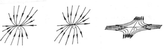
( a ) ( b ) ( c )
Figure 13.1
2 ¡ã eigenroots are complex numbers:
![]()
The general solution is in the form of
where c 1 , c 2 are arbitrary constants, and c 1 *, c 2 * are linear combinations of c 1 , c 2 .
( i ) 1 ,2 = p iq , p <0, q 0.
The zero solution is stable . The orbital shape is shown in Figure 13.2( a ). This type of equilibrium point ( 0,0) is called a stable focus .
( ii ) 1 ,2 = p iq , p >0,
q 0.
The zero solution is unstable . The orbital shape is shown in Figure 13.2( b ). This type of equilibrium point ( 0,0) is called an unstable focus .
( iii ) 1 , 2 = iq , q 0.
The zero solution is stable . The orbital shape is shown in Figure 13.2( c ). This type of equilibrium point ( 0,0) is called the center, and the center is stable .
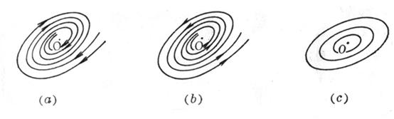
Figure 13.2
The 3 ¡ã characteristic equation has multiple roots:
![]()
The general solution is in the form of
( i ) 1 = 2 < 0
The zero solution is asymptotically stable . The orbital shape is shown in Figure 13.3( a ). This type of equilibrium point ( 0,0) is called a stable degenerate node .
If the zero solution is a stable node, it is called a critical node . The shape of the orbit is shown in Figure 13.3 ( b ).![]()
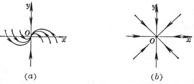
Figure 13.3
( ii ) 1 = 2 > 0
The zero solution is unstable . The orbital shapes are shown in Figure 13.3 ( a ) and ( b ), but the arrows are in opposite directions . This type of equilibrium point (0,0) is called the unstable degenerate node and the unstable critical node .
Combining the above situations, the following conclusions can be drawn: if the roots of the characteristic equation have negative real parts, then the zero solution is stable and asymptotically stable; if the characteristic equation has a root with a positive real part, then zero The solution is unstable .
This conclusion, for the general system of homogeneous linear differential equations with constant coefficients
![]()
is also established .
Theorem if the characteristic equation of a system of homogeneous linear differential equations with constant coefficients
A zero solution is asymptotically stable if all roots have negative real parts; a zero solution is unstable if at least one of all the roots of the characteristic equation has a positive real part .
[ Determining stability by first approximation ] Consider the system of equations
![]()
where a ij ( i , j =1,2, ¡ , n ) is a constant, and R i ( x 1 , x 2 , ¡ , x n ) ( i = 1,2, ¡ , n ) is a constant for lower than the second order .![]()
Its first-order approximate equation system is
![]()
Stability can be determined by studying various cases of the characteristic roots i ( i = 1,2, ¡ , n ) of a system of first-order approximate equations . There are two basic theorems:
The first theorem If all the eigenvalues of the first approximation equation system have negative real parts, then the zero solution of the original equation system is asymptotically stable .
The second theorem If at least one of the eigenvalues of the first-order approximate equation system has a positive real part, then the zero solution of the original equation system is unstable .
These two theorems cover all stable cases (called noncritical cases) in which the zero solution of the original system of equations can be studied with a first-order approximation . As for at least one root with a zero real part, all other roots have negative In the critical case of the real part, the higher-order terms on the right-hand side of the equation system play an important role in the stability of the zero solution, so it is generally impossible to study the stability problem by the first-order approximation equation system .
[ Hurwitz Discriminant Method ] It is a method to directly use some properties of the determinant formed by the coefficients of the characteristic equation to determine the stability of the zero solution of a system of linear differential equations with constant coefficients .
Let the characteristic equation of the system of linear differential equations with constant coefficients be
![]()
Then the necessary and sufficient conditions for the zero solution of the system of constant coefficient linear differential equations to be asymptotically stable are: a 0 >0 , and all Hurwitz determinants
are all positive (the final ¦¤ n > 0 can be replaced by the condition a n > 0 ) .
If ¦¤ n =0 , then since ¦¤ n = a n ¦¤ n -1 =0 , there must be an =0 or ¦¤ n -1 = 0 . If an = 0 , the characteristic equation has zero roots; if ¦¤ n -1 = 0 , then the characteristic equation has pure imaginary roots, in both cases the zero solution may or may not be stable .
The characteristic equation is the Hurwitz discriminant condition for quadratic, cubic and quartic (for the convenience of drawing, a 0 =1 is taken below ):
( i ) Characteristic equation:![]()
Hurwitz conditions are a 1 >0,
a 2 >0
The stable region is shown in Figure 13.4( a ).
( ii ) Characteristic equation:![]()
The Hurwitz condition is ![]()
The stable region is shown in Figure 13.4( b ).
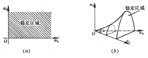
Figure 13.4
( iii )
Characteristic equation:![]()
The Hurwitz condition is . ![]()
[ Lyapunov's second method (direct method) ] to study systems of differential equations
![]() (1)
(1)
There is a more general method for the stability of the equilibrium point of , the so-called Lyapunov method .
1 ¡ã Lyapunov stability theorem For the system of equations (1) , if one can find a differentiable function V ( x 1 , x 2 , ¡ , x n ) (called the Lyapunov function ) that satisfies the following conditions in the neighborhood of the origin ):
( i ) V ( x 1 , x 2 , ¡ , x n ) ¡Ý 0 (or ¡Ü 0 ), and only when x i =0 ( i =1,2, ¡ , n ) , V =0 .
( ii ) When t ¡Ý t 0 , the full derivative of V along the integral curve of the system of equations ( 1)
![]() ( or )
( or )![]()
Then the equilibrium point x i =0 ( i =1,2, ... , n ) of the system of equations (1 ) is stable .
2 ¡ã Lyapunov Asymptotic Stability Theorem For the system of equations (1) , if one can find a differentiable function V ( x 1 , x 2 , ¡ , x n ) in the neighborhood of the origin that satisfies the following conditions (called Lyapunov Nov function):
( i ) V ( x 1 , x 2 , ¡ , x n ) ¡Ý 0 (or ¡Ü 0 ), and only when x i =0 ( i =1,2, ¡ , n ) , V =0 .
( ii ) The total derivative along the integral curve of the system of equations ( 1)
![]() ( or )
( or )![]()
And outside a suitably small delta neighborhood of the origin (ie ), when t ¡Ý t 0 , (or ) then the equilibrium point x i =0 ( i =1,2, ¡ , n ) of the system of equations (1 ) is asymptotically nearly stable .![]()
![]()
![]()
Case Study of Differential Equations
Stability at the equilibrium point x = 0, y = 0 .
The characteristic equation of the first-order approximation equation for solving this system of equations has two pure imaginary roots, so it is a critical case and cannot be studied by the first-order approximation method . Now use the Lyapunov method . Take
![]()
because
( i ) ![]()
( ii ) ![]()
For any ¦Ä > 0 , when t > t 0 , . Therefore, the equilibrium point (0,0) is asymptotically stable .![]()
![]()
3. Limit cycle (or limit cycle)
Only the case of n = 2 is discussed here .
[ periodic solution ] equation

A periodic solution with period T is a solution that satisfies x ( t + T ) = x ( t ) and y ( t+T ) = y ( t ) . The orbit corresponding to the periodic solution is a closed curve . Conversely, a closed orbit corresponds to the periodic solution .
[ Limit cycle ] The isolated periodic solution is called the limit cycle of the equation . In a complete way , it is: let x=x ( t ), y=y ( t ) be the periodic solution of the equation, and K is the solution drawn on the phase plane The closed curve of . If there is a positive number ¦Ñ , such that for any point ¦Æ on the phase plane whose distance from K is less than ¦Ñ , the solution of the equation through the point ¦Æ is not periodic, then x=x ( t ) , y=y ( t ) (that is, the closed orbit K ) is an isolated periodic solution, or a limit cycle .
example
Do coordinate transformation: x = r cos , y = r sin ![]()
![]() , the equations are transformed into
, the equations are transformed into
![]()
The general solution is
|
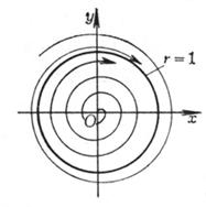
Figure 13.5 |
Where k , t 0 are arbitrary . Take t 0 =0 , then the solution of the system of equations is
When k= 0 , it is a circle x 2 + y 2 =1 ; when k=c 2 ( c> 0) , it is a spiral, when t - , it tends to the origin, and when t , it is approached from the inner spiral Circumference x 2 + y 2 =1 ; when k= ( c> 0) , the orbit is a curve, when t log c +0 , it tends to infinity, and when t , it circles from the outside to approximate the circumference x 2 + y 2 =1.
![]()
The track distribution is shown in Figure 13.5.
Then the circumference x 2 + y 2 =1 is the only limit cycle of the system of equations . (0,0) is the only singular point .
[ Limit cycle existence theorem ] For the system of equations
1 ¡ã There are two simple closed curves C 1 and C 2 on the xy plane ,
C 2 is inside C 1 , and the following two conditions are satisfied:
( i ) The vector field of a point on C1 points from the outside of C1 to the inside, and the vector field of a point on C2 points from the inside of C2 to the outside ;
( ii ) There is no singularity in the system of equations in the annular region enclosed by C 1 and C 2 ;
Then in the annular region enclosed by C 1 and C 2 , there must be a stable limit cycle (called the Poincare - Bendikesen theorem) .
2 ¡ã If in a simple connected region G , the sign is constant, and it is not equal to zero in any subregion D ( G ) , then in G , the system of equations does not have any closed orbits . ©¡ ![]()