§ 6 Numerical solution of ordinary differential equations
1. Numerical solution of the initial value problem of first-order differential equations
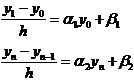
require differential equations
![]()
in the initial condition
![]()
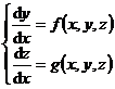
The numerical solution below is to be a series of points in the interval where the solution exists
![]()
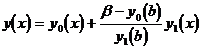
Starting from the initial value y 0 , the approximate value is calculated one by one .![]()
![]()
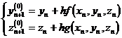
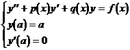
[ Improved Euler method (prediction correction method) ] The calculation formula is
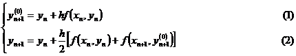
where y n represents the approximate value of y ( x n ) and represents the step size . Here the truncation error is![]()
![]()
In this method, formula (1) uses the broken line method to provide the initial value, which is called the forecast formula . The formula (2) uses the trapezoidal method to give a more accurate value, which is called the correction formula . Collectively, it is called the forecast correction formula .
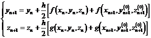
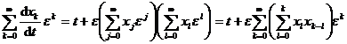
[ Runge - Kutta method ] calculation formula is
![]()
in the formula
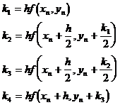
The truncation error is R=O ( h 5 )
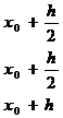
When calculating by hand, proceed from top to bottom according to the table .
|
|
|
|
k |
|
x 0
|
y 0
|
|
|
[ Adams Method ]
1 ° interpolation formula
![]()
This is an implicit equation for , which can be solved iteratively as long as h is small .![]()
2 ° extrapolation formula
![]()
This is an explicit equation for y n +1 , and y n +1 can be calculated directly from the formula as long as the values of the first few points are known .
3 ° Forecast Correction Formula
The truncation error is
R=O ( h 5 )
The Adams method can be calculated by the extrapolation formula alone. For each calculation of y n +1 , the value of f ( x, y ) only needs to be calculated once , and the calculation amount is smaller than that of the Runge - Kutta method, and the truncation error is the same order, so The small amount of calculation is one of the advantages of the extrapolation method . The disadvantage is that the first few y i values cannot be calculated by this method, and other methods (generally the Runge - Kutta method can be used) are required to calculate y 1 , y 2 , and y 3 .
Supplementary explanation In the 1 ° Adams method, the calculation of the value of y n +1 is called the multi-step method . The improved Euler method and Runge - Kutta method only need to use y n , so it is called for the one-step method . ![]()
2 ° It is convenient to change the step length in the one-step method, and it is troublesome to change the step length in the multi-step method, because the first few items must be recalculated in the one-step method .
Another advantage of the 3 ° multi-step method is that the truncation error can be estimated by the way .
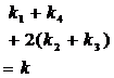
Use y n +1 ( E ) and y n +1 ( I ) to denote the values calculated by the extrapolation and interpolation formulas, respectively, there are
![]()
In the formula . If the allowable error specified in the calculation does not exceed ε , then ε and
![]()
For comparison, if , the calculation can be continued, otherwise the error is too large, and the step size should be reduced . If it is much smaller than ε , the step size may be enlarged to improve the calculation speed .![]()
![]()
Second, the numerical solution of the initial value problem of the first-order differential equation system
For the sake of simplicity, only the differential equation system with two unknown functions and the differential equation system with multiple unknown functions are discussed, and the calculation formulas are similar .
and initial conditions
![]()
[ Improved Euler method (prediction correction method) ]
forecast formula
Correction formula
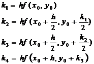
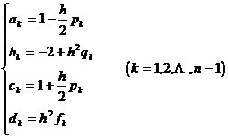
[ Runge - Kutta method ] calculation formula is
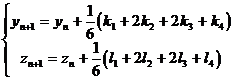
in
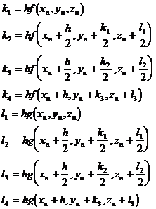
Calculate first and then calculate y n +1 , z n +1 .![]()
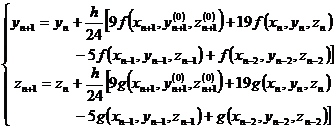
[ Forecast correction formula for Adams method ]
Forecast value (extrapolation formula)
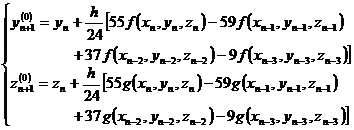
Correction value (interpolation formula)
The computation of the first few y j and z j is the same as the Runge - Kutta method in Section 1 .
3. The boundary value problem
Only the boundary value problems of second-order linear ordinary differential equations are discussed here .
 (1)
(1)
[ Difference method ] Divide the interval [ a, b ] into n equal parts, the step size , and the points x 0 = a , x 1 = a+h ,
… ,
x k = a+kh ,
… , x n = b are called Node . The differential quotient is replaced by the difference quotient, and the boundary value problem is transformed into the solution of the following system of difference equations .
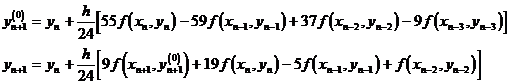
![]()
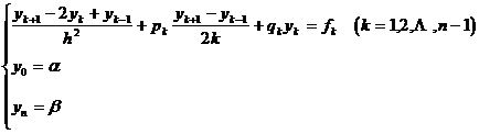
where y k = y ( x k ), p k = p ( x k ), q k = q ( x k ), f k = f ( x k )
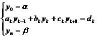
( ). ![]() The above system of difference equations can be viewed as n + A linear algebraic equation system with unknown quantities y 0 , y 1 , y 2 , … , y n , the number of equations is also n +1 . After sorting and merging similar items, the difference equation system can be rewritten as
The above system of difference equations can be viewed as n + A linear algebraic equation system with unknown quantities y 0 , y 1 , y 2 , … , y n , the number of equations is also n +1 . After sorting and merging similar items, the difference equation system can be rewritten as
 ( )
( )![]()
in the formula
This is a special form of linear algebraic equations , in addition to the elimination method, iterative method, etc. can be used to solve, but also a simpler and more effective method - the chasing method ( see Chapter 4 , § 3).
In applications, boundary conditions of the following form may also be encountered:
where α 1 , α 2 , β 1 , β 2 are known constants . At this time, the two equations corresponding to the boundary conditions in the above differential equation system should be replaced by:
[ Turn into a numerical solution to the initial value problem ] First solve the initial value problem
The numerical solution y 0 ( x ) of , and then the corresponding homogeneous equations that satisfy the initial conditions y ( a )=0, y' ( a )=1
![]()
The numerical solution y 1 ( x ) of . The solution of the original boundary value problem (1) can be expressed as
Fourth, the small parameter method
When the differential equation contains a parameter ε with a small absolute value, the method of writing the solution as a power series of ε to obtain an approximate analytical solution is called the small parameter method . The initial value problem of ordinary differential equations is briefly introduced below .
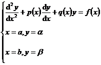
Given a system of differential equations
![]() (1)
(1)
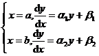
Assume that all functions of as t are sufficiently smooth, as functions of as analytic, and can be expanded into a power series of ε at ε = 0![]()
![]()
![]()
The coefficients are all analytic functions of x 1 , … , x n .![]()
given the initial conditions
When t=t 0 , x i = x i ( ε ) = x i (0) + ε x i (1) + …
(2)
So the solution of equation system (1) that satisfies the initial condition (2) exists in a certain region of t and ε , and can be expanded into a power series of ε
![]() (3)
(3)
And any partial sum of (3 ) is the approximate analytical solution of (1) that satisfies (2) . In the specific calculation, it is only necessary to substitute the series (3) into (1) , and convert both sides into the power series of ε shape, and then compare the coefficients .
Example to find the Riccati equation with small parameter ε
![]()
meet the initial conditions
t= 0, x= 0
solution .
De- assign
![]()
Substituting into the above differential equation, we get
which is
![]()
Let the coefficients of the same power of ε on both sides be equal, we get
In addition, the initial conditions can be rewritten as
![]()
So it can be listed
find out
and
![]()
is the approximate expression being solved (that is, the approximate analytical solution) .