4. Regression Analysis

 

1. The principle of least squares

   Let u be a function of variables x , y ,... , with m parameters a ₁ , a ₂ ,..., a _m , namely

                u =f ( a ₁ , a ₂ ,..., a _m ; x , y ,...)

Now make n observations of u and x , y , . . . ( x _i , y _i , . . . ; u _i )( i = 1,2, . . . , n ) . So the absolute error between _the theoretical value of u and the observed value ui is

                      ( i = 1,2,..., n )

The so-called least squares method is to require the above n errors in the sense of the smallest sum of squares, so that the function u =f ( a ₁ , a ₂ ,..., a _m ; x , y ,... ) and the observed value u ₁ , u ₂ , ... , u _{n is} the best fit. That is, the parameters a ₁ , a ₂ ,... , a _m should be

               minimum

According to the method of finding the extreme value of differential calculus, it can be known that a ₁ , a ₂ , ··· , a _m should satisfy the following equations

                    ( i = 1,2,..., n )

2. Univariate Linear Regression

[ Univariate regression equation ]   The observed value corresponding to the independent variable x and the variable y is

If there is a linear relationship between the variables, a straight line can be used

to fit the relationship between them. By the least squares method, a , b should be

minimum

have to

in the formula

   

   

The equation is called the regression equation (or regression line), and b is called the regression coefficient.

[ Correlation coefficient and its test table ] The   correlation coefficient r _xy reflects the closeness of the linear relationship between the variables x and y , which is defined by the following formula

in

(In the absence of misunderstanding, r _{x y} is abbreviated as r ). Obviously . At that time , it is called complete linear correlation; at that time , it is called complete wireless correlation; when it is closer to 1 , the linear correlation is greater.

   The following table gives the minimum value of the correlation coefficient (it is related to the number of observations n and the given reliability ), when it is greater than the corresponding value in the table, the matching straight line is meaningful.

N — 2	= 5 %	= 1 %	n -2	= 5 %	= 1 %	n- 2	= 5 %	= 1 %
1 2 3 4 5 6 7 8 9 10 11 12 13 14 15	0.997 0.950 0.878 0.811 0.754 0.707 0.666 0.632 0.602 0.576 0.553 0.532 0.514 0.497 0.482	1.000 0.990 0.959 0.917 0.874 0.834 0.798 0.765 0.735 0.708 0.684 0.661 0.641 0.623 0.606	16 17 18 19 20 twenty one twenty two twenty three twenty four 25 26 27 28 29 30	0.468 0.456 0.444 0.433 0.423 0.413 0.404 0.396 0.388 0.381 0.374 0.367 0.361 0.355 0.349	0.590 0.575 0.561 0.549 0.537 0.526 0.515 0.506 0.496 0.487 0.478 0.470 0.463 0.456 0.449	35 40 45 50 60 70 80 90 100 125 150 200 300 400 1000	0.325 0.304 0.288 0.273 0.250 0.232 0.217 0.205 0.195 0.174 0.159 0.138 0.113 0.098 0.062	0.418 0.393 0.372 0.354 0.325 0.302 0.283 0.267 0.254 0.228 0.208 0.181 0.148 0.128 0.081

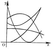
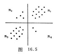   Note that when the number of observations n is large , the correlation coefficient can be approximated by the following method: Plot the pair of observations ( x _i , y _i ) ( i =1,2,..., n ) on the coordinate paper, First, make a horizontal line to make the upper and lower points of the line equal, and then make a vertical line to make the left and right points equal. These two lines (try to make no points on the two lines) divide the plane into four pieces (Figure 16.5 ) and set it to the upper right square , upper left , lower left and lower right points are n ₁ , n ₂ , n ₃ , n ₄ respectively , let

n ₊ =n ₁ +n ₃          =n ₂ +n ₄

Then the correlation coefficient is approximately                                                                        

 

 

 

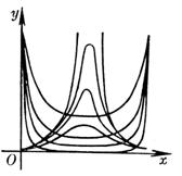
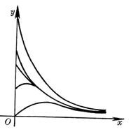
[ Remaining Standard Deviation ]

           

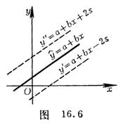
Called the residual standard deviation , it describes the precision of the regression line : for each x of the experimental range , 95.4% of the y values ​​fall on two parallel lines

  

between ( Fig. 16.6 ); 99.7% of the y values ​​fall between two parallel lines

 

between .

[ Calculation steps of unary regression ]   For the convenience of calculation , rewrite l _xx , l _yy , l _xy as                                                                               

and integerize the data . That is

  

    After integerization , we have

             ,  

                

So the list is calculated as follows :

serial number
1   2     n
mark				=	= -	= -	= -
		count Calculate Knot fruit	Regression coefficients  Constant term    regression equation  Correlation coefficient  residual standard deviation

[ _Analysis of variance for univariate linear regression ] The independent   variable x is regarded as a single factor , and the data y _ij ( i = 1,2 , , n ; j = 1,2, , k ) , recorded as follows :

	y ij
x 1                x 2 x n	y 11   y 12 y 1 k _    y 21   y 22 y 2 k _            y n 1   y n 2 y nk _

Find the regression equation in pairs      

The total sum of squares of y is

        

Referred to as

                 

The S on the right side of the above is _{called the} regression _sum of squares , which is caused by the change of x , which also changes y ; , it is caused by other random factors or an inappropriate fit of the regression line .

   Similar to the one-way ANOVA , the one-way linear regression ANOVA table is as follows : 

source of variance	sum of square	degrees of freedom	mean square	Statistics	confidence limits	statistical inference
return     remaining     error	S back     S Yu     S error	k     n     n	s back			At that time , the impact was considered insignificant; At the time , the impact was considered significant
total sum of squares	S total	nk

   During the test , if the effect is not significant, it indicates that the residual sum of squares is basically caused by random factors such as experimental error; if the effect is significant, it indicates that there may be other factors that cannot be ignored, or x and y are not linearly related, or x and y It doesn't matter. At this time, the regression line obtained cannot describe the relationship between x and y , and it is necessary to further identify the cause and re-wiring.

   During inspection , if the influence is significant, it indicates that there is a linear relationship between x and y ; if the influence is not significant, rewiring is required.

   S _total , S _return , S _remainder , and S _error are calculated according to the following formulas (the data can be integerized first , :

S _total =

S _back =

S _surplus =

S _error = S _{total return surplus}

in the formula

3. Parabolic regression

   Given a set of observations ( x _i , y _i ) ( i = 1,2,..., n ) , if there is a parabolic relationship, a polynomial of degree m ( m 2 ) can be used

to fit. According to the principle of least squares, the

= minimum value

    In particular, if p(x) is taken as a quadratic polynomial

                    

Then the coefficients a , b , c satisfy the equations

in the formula

   

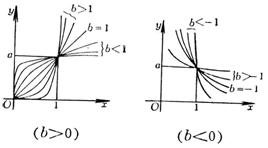
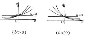
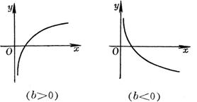
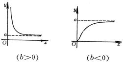
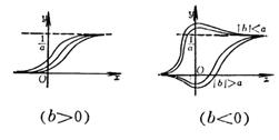
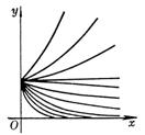
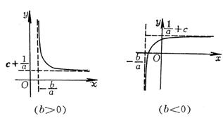
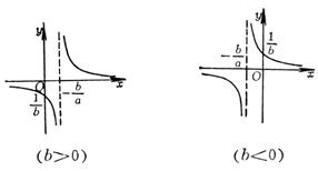
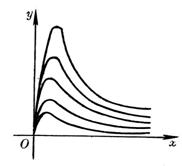
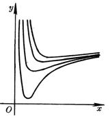
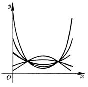
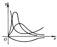
4. Curve regression that can be transformed into linear regression

   If the number of observations forms a curve against the distribution on the graph paper, appropriate variable substitutions can be made to perform a linear regression on the two new variables. Then restore to the original variable.

Common curve types that can be straightened

 

 

 

 

 

 

 

Curve type		Linearized variable substitution
1 °		Assume but ( x , y ) is a straight line on double logarithmic paper
		Let X = x , Y = but ( x , y ) line up on logarithmic paper
		Assume but ( x , y ) line up on logarithmic paper
		Assume    but
		Assume    but
	The curve is the same as the type, but moved in the direction of the axis. First, take three points on the given curve: , , ), then	After c is determined, set      but
curve	type	Linearized variable substitution
	The curve is the same as the type, but moved in the direction of the axis, first take three points on the given curve:  but	After confirming, set           but
		Assume    but
		Assume    but
		Take a point on the curve ( x 0 , y 0 ) Let X = x   but Using the regression line method, A and B can be determined from the given data
		Take a point on the curve ( x 0 , y 0 ) Let X = x   but
Curve type		Linearized variable substitution
		Let X = x   can be transformed into type 11 °
		Let X = x   Y = y 2 can be transformed into type 11 °
		Let X = x   can be transformed into type 11 °
		Assume    can be transformed into type 11 °
		Let X = x   but Converted to Type 11 °
		If the given x values ​​form an arithmetic progression with h as tolerance, then let (value ) (value ) straight
		If the given x value constitutes an arithmetic series with h as the tolerance, let u 1 = x+h , u 2 = x+ 2 h , and the corresponding y values ​​are v 1 , v 2 set again and get Then use the regression line method to determine b and d , then set      then get

 

5. Binary line regression

[ Regression equation ] The values ​​corresponding to   the values ​​of the independent variables x ₁ and x ₂ are , so n points are obtained , and the regression equation is

where is the regression coefficient, which is determined by the following equation:

here    

And where is the data transformation (without integerization) to simplify the calculation, that is

( 1 ) The constant term in the formula

[ Multiple correlation coefficient and partial term correlation coefficient ]

is called the complex correlation coefficient, where

Here it is shown in (2) . The complex correlation coefficient R is satisfied , and its meaning is similar to the correlation coefficient r in the single linear regression analysis, which is used to measure the closeness of the linear relationship between y and x ₁ , x _{2 .}

    If you only want to express the correlation between y and one of the variables ( x ₁ or x ₂ ) , then you must remove the influence of the other variable and then calculate their correlation coefficient, which is called the partial correlation coefficient. The correlation coefficient of x ₁ , y after removing the influence of x ₂ is called the partial correlation coefficient of x ₁ , y to x ₂ , denoted as , it can be expressed by ordinary correlation coefficient :

Similarly, the partial correlation coefficient table for the pair is

[ Remaining Standard Deviation ]

It is called the residual standard deviation, and its meaning is similar to the residual standard deviation s in the linear regression analysis .

[ Standard regression coefficient and partial regression sum of squares ]   When the relationship between the two factors x ₁ and x ₂ is not close, the following method can be used to determine which factor is the main one.

1 ^°                           

                                                     

It is called the standard regression coefficient, where b ₁ , b ₂ are regression coefficients, l ₁₁ , l ₂₂ are shown in ( 2 ) , and l ₀₀ is shown in ( 4 ) . If , it indicates that among the two factors affecting the variable, x ₁ is the main factor and x ₂ is the secondary factor.

   2 ^°                       

                                                   

It is called partial regression sum of squares, where b ₁ , b ₂ are regression coefficients, and l ₁₁ , l ₁₂ , and l ₂₂ are shown in (2) . If p ₁ >p ₂ , it means that x ₁ is the main factor, and x ₂ is the secondary factor.

[ t -value ]

  

They are called the t values ​​of x ₁ and x ₂ , respectively, where s is the residual standard deviation, and p ₁ and p ₂ are the partial regression sums of squares. The larger the t value, the more important the factor is. According to experience, when t _i > 1 , the factor x _i has a certain influence on y ; when t _i > 2 , the factor x _i is regarded as an important factor; when t _i < 1 , the factor x i is considered to be an important factor _i has little effect on y and can be ignored and does not participate in the regression calculation.

[ Binary Linear Regression Calculation Table ]   x _{k i} in the table is the simplified data.

sequence No	x 1 i		y i	x	x
1   2 n	x 11   x 12 x 1 n	x 21   x 22 x 2 n	y 1   y 2 y n
			Knot fruit

From , according to ( 2 ) and ( 3 ) are calculated respectively , get the regression equation

                       

And continue to calculate the complex correlation coefficient R , the standard regression coefficients B ₁ and B ₂ , the partial regression square sum p _{1 ,} , p ₂ , and the t values ​​t ₁ and t ₂ , and perform binary regression analysis based on these data.

    Regarding the binary nonlinear regression problem, appropriate variable substitution can be done to form a linear relationship between the new variables, and then the regression analysis can be performed.

6. Multiple linear regression

   Consider the relationship between the independent variable and the dependent variable y , do n experiments, and the observed value is, let ; , let

  

   

       

set the matrix again

Its inverse matrix is

[ regression equation ]

where is the regression coefficient, which is represented by a vector as

b

in

Constant term

[ Multiple Correlation Coefficient ]

[ Remaining Standard Deviation ]

[ ANOVA table for multiple linear regression ]

variance source	sum of square	degrees of freedom	mean square	Statistics _	confidence limits	statistical inference
back    return    leftover    Remain		m           nm- 1				At that time , the regression was considered significant and the linear correlation was close; At that time , the regression was considered insignificant and the linear correlation was not close.
total flat Fang He		n- 1

 

[ Standard regression coefficients and partial regression sum of squares ]

Standard regression coefficients         

Partial regression sum of squares            

[ t -value ]

      

   The multiple linear regression analysis is similar to the binary case, but the calculation amount is larger and can be done with the help of an electronic computer.