V. Orthogonal experimental design

 

[ Orthogonal Table and Orthogonal Test ]   Orthogonal table is a table constructed according to the combination theory and certain rules, and it is widely used in experimental design. An experiment that uses the orthogonal table as a tool to arrange the test plan and analyze the results is called an orthogonal test. It is suitable for experiments with multiple factors, multiple indicators (the results that the experiment needs to examine), there is interaction between multiple factors (the factors work together), and there are random errors. Through the orthogonal test, the influence of each factor and its interaction on the test index can be analyzed, the primary and secondary relationship can be found according to its importance, and the optimal process conditions for the test index can be determined. Each factor considered is required to be controllable in an orthogonal test. The number of values ​​taken by each factor in the whole experiment is called the level of the factor.

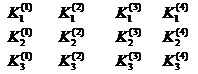
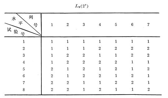
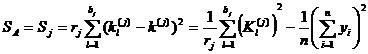
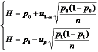
The symbol of the orthogonal table is , which represents the orthogonal table; the subscript is the number of rows in the orthogonal table, indicating the number of experiments; the number of columns in the orthogonal table, indicating the maximum number of factors that can be arranged in the experiment; the different numbers in the table , indicating the number of levels for each factor. For example , 8 means that there are 8 rows in the orthogonal table , that is, the number of trials is arranged 8 times; 7 means that there are 7 columns in the orthogonal table, and experiments can be arranged for up to 7 factors (including interaction factors); 2 means that each The factor has only two levels. Such an orthogonal table is called a 2 -level orthogonal table.

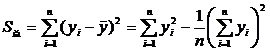
For another example , it means that there are 12 rows and 4 columns in the orthogonal table , one of which is 3 - level, and 3 of which are 2 -level. It is called a mixed-type orthogonal table and can be used to arrange experiments with different levels of factors.

[ Interaction Column of Orthogonal Table ]   After two factors are arranged in any two columns, the interaction of these two factors can be shown in other columns of the table, which are called interaction columns. The interaction column has only one column in a 2-level orthogonal table, and two columns in a 3 -level orthogonal table, for example , the interaction column of any two columns is the other two columns. Usually low-level (the number of levels is 2 or 3 ) orthogonal table has another table to write the interaction column, such as the interaction list, indicating that the interaction column of the 3rd column and the 5th column is the 6th column and so on. For some orthogonal tables, for example , the interaction column of any two columns is not in the table, and the interaction between factors cannot be considered for such orthogonal tables.

    Commonly used quadrature tables are available at the back of the manual.

 interactive list of

1    2    3    4    5    6    7	column number
( 1 ) 3    2    5    4    7    6      ( 2 ) 1    6    7    4    5          ( 3 ) 7    6    5    4              ( 4 ) 1    2    3                  ( 5 ) 3    2                      ( 6 ) 1                          ( 7 )	1 2 3 4 5 6 7

[ Orthogonality of Orthogonal Tables ]   Orthogonal tables have orthogonality :

    1 ^° In any column, each level is repeated an equal number of times, e.g. 4 repetitions for each level in each column .

    2 ^° In any two columns, the number pairs formed by the same number (level) contain all possible (under this level) number pairs , and each number pair is repeated the same number of times . For example , the number pair formed by any two columns in , contains all possible number pairs under 3 levels: ( 1 , 1 ), ( 1 , 2 ), ( 1 , 3 ), ( 2 , 1 ), ( 2 , 2 ) ), ( 2 , 3 ), ( 3 , 1 ), ( 3 , 2 ), ( 3 , 3 ), and each pair is repeated equal to 1 .

    Due to the orthogonality, the arranged orthogonal tests are evenly dispersed and neatly comparable.

[ Formulation steps and arrangement method of the experimental plan ]

   1 ^° step

    ( 1 ) Determine the number of change factors in the experiment and the level of change of each factor.

    ( 2 ) Based on professional knowledge or experience , preliminarily analyze the interaction between various factors to determine which ones must be considered and which ones can be ignored temporarily

    ( 3 ) According to the manpower, equipment, time and cost of the test, determine the approximate number of tests that may be carried out.

    ( 4 ) Select a suitable orthogonal table and arrange the test.

   2 ^° Arrangement method 

    ( 1 ) Arrange the factors in any column of the orthogonal table one by one without considering the interaction, then the experimental conditions (the level that each factor should take) of each experiment (corresponding to the row of the orthogonal table) are arranged by The level of each column of the factor is determined.

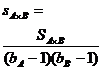
    For example, in the process of making beer with unmalted barley, four factors were selected, each with three levels, and the indicator was powdery ( % ) .

factor level table

 

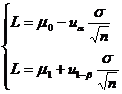
factor level	Bottom water ( A ) Ammonia soaking time ( B ) 920 concentration ( C ) Ammonia concentration ( D )
1    2    3	A 1 (140) B 1 (180) C 1 (2.5) D 1 (0.25)                     A 2 (136) B 2 (215) C 2 (3.0) D 2 (0.26)                     A 3 (138) B 3 (250) C 3 (3.5) D 3 (0.27)

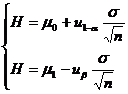
If the interaction is not considered, the orthogonal table can be used , and the experimental scheme is as follows:

               

Arrange a four-factor experimental protocol with

 

column number (factor) test number

1( A )    2( B )    3( C )    4( D )

1      2      3      4      5      6      7      8      9

1( A 1 )   1( B 1 )    1( C 1 )   1( D 1 )   1( A 1 )   2( B 2 )    2( C 2 )   2( D 2 )   1( A 1 )   3( B 3 )    3( C 3 )   3( D 3 )   2( A 2 )   1( B 1 )    2( C 2 )   3( D 3 )   2( A 2 )   2( B 2 )    3( C 3 )   1( D 1 )   2( A 2 )   3( B 3 )    1( C 1 )   2( D 2 )   3( A 3 )   1( B 1 )    3( C 3 )   2( D 2 )   3( A 3 )   2( B 2 )    1( C 1 )   3( D 3 )   3( A 3 )   3( B 3 )    2( C 2 )   1( D 1 )

This table indicates that the condition of Test No. 1 is, and the condition of Test No. 2 is the condition of Test No. 9 .

   ( 2 ) When the interaction needs to be considered, the factors cannot be arranged arbitrarily, and the corresponding table header design should be used to arrange the test. At this time, it should be noted that different factors (including the considered interaction) cannot be placed in the same column ( because the different effects of the same column cannot be analyzed in the analysis ) . If this is not possible, a larger positive value should be used. Submit the form. For example, to arrange an experiment with four factors A , B , C , D , interactions must be considered , and other interactions can be ignored. According to the header design:

 

 

column number number of factors	1       2       3       4       5       6       7
3	A       B     C
4	A       B     C
4	A
5

Because it is a four-factor experiment, A , B , C , and D can be arranged on the 1st , 2nd, 4th, and 7th columns respectively , and the 3rd and 5th columns respectively represent and , and the 6th column is empty. If all the interactions of the four factors A , B , C , D should be considered, it cannot be used , and a larger orthogonal table should be used, eg . 

[ Intuitive Analysis of Orthogonal Tables ]   1 ^° Calculate the level and K _i of the i -th level and the level average value k _i. For example, with the arrangement of the four-factor and 3 - level test plan, the intuitive analysis table can be listed as follows:

column number (factor) test number	1( A )   2( B ) 3( C ) 4( D )	Test index y
1       2       3       4       5       6       7       8       9	1     1      1      1     1     2      2      2     1     3      3      3     2     1      2      3     2     2      3 1          2     3      1      2     3     1      3      2     3     2      1      3     3     3      2      1	y 1    y 2    y 3    y 4    y 5    y 6    y 7    y 8    y 9
K 1             K 2             K 3
k 1              k 2            k 3
Range R	R (1)     R (2)    R (3)     R (4)

in

    Indicates the test index sum of the i level in the jth column (abbreviated as the level sum)

    Represents the mean value of the test index of the i level in the jth column (referred to as the level mean)

    represents the range of the jth column

E.g

 

  2 ^{° The} importance order of the evaluation factors is ranked according to the range of the average value of each factor index  , and the larger range indicates that the factor is important.

  3 ^{° After} drawing the relationship diagram of each factor and the test index ,  for each j , use the horizontal value i as the abscissa and ki as the ordinate to draw the point and draw a line graph, which is called the jth _factor and the test index. relation chart. If the variation of k _{i is large, the influence of the corresponding factor will be greater.} If the points depicted on the graph are scattered, it means that the factor is primary; if the points are concentrated, it means that the factor is secondary.

    When the interaction of factors needs to be considered, the ki column corresponding to a certain interaction _indicates that it is caused by the influence of the interaction. The interaction between the factors and the relationship between the experimental indicators can also be plotted.

    For "empty columns" where neither factors nor interactions are arranged, estimates of experimental error can be arranged. The k _i is obtained by the same calculation , which can be regarded as due to the experimental error, and the magnitude of the change in k _i reflects the size of the experimental error. The relationship between the experimental error and the experimental index can also be drawn.

  4 ^° Choose the optimal process conditions (optimal matching scheme )   without considering the interaction , just according to the requirements of the test index (that is, whether the index is higher is better, or lower is better), from each Find the level of the optimal point (the highest point or the lowest point) in the relationship diagram of the factors, and combining the optimal levels of each factor is the optimal process condition for the index.

  When the interaction between factors needs to be considered, it is known that the interaction of a certain two factors has a great influence on the test index. If there are multiple trials of the same combination, the average value should be calculated) for comparison, and the optimal level combination of the two factors should be selected. Finally, the optimal conditions selected by combining other factors or interactions are considered comprehensively to determine the optimal process conditions.

    For multi-index experiments, each index can be analyzed as above. The optimal process conditions should be determined according to the comprehensive consideration of each index.

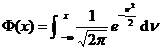
[ Analysis of Variance in Orthogonal Tables ]   Suppose factor A is arranged in the jth column of the orthogonal table, the number of levels in this column is b _j (or b _A ), the number of repetitions for each level is r _j , and the number of trials is n (the number of rows) (obviously r _j b _j =n ), then the sum of squares of factor A S _A (or called the j -th column sum of squares S _j ) is

The total sum of squares is

             

    The sum of squares of non-negligible interactions is also calculated according to the sum of squares of its column (the formula is the same as the formula for calculating the sum of squares of factor A ₎ .

    The error sum of squares is equal to the difference of the sum of squares of the columns with all arrangements that have factors or interactions , i.e.

               

 

ANOVA Table for Orthogonal Tables

dispersion source	sum of square	degrees of freedom	mean square	Statistics	confidence limits	statistical inference
A      B            error	S A     S B	b A – 1     b B – 1           n is wrong				At that time , the corresponding factors were considered to have a significant impact; At that time , the corresponding effect was considered to be insignificant
total flat Fang He		n

   table

            

   The analysis of variance on the orthogonal table can quantitatively give the primary and secondary relationship of the factors, and can judge which factors are important factors and which factors are secondary factors. At this time, the determination of the optimal process conditions only needs to consider important factors, as for the level of those secondary factors, it can be determined according to other conditions.

 

6. Sampling inspection method

 

[ Type 1 and Type 2 errors in sampling acceptance ]   There may be two kinds of errors when randomly selecting n samples from the whole batch of products for quality inspection, and then making the judgment of "acceptance " or "rejection " of the whole batch of products : The whole batch of products that can be accepted is wrongly judged as unqualified and "rejected " , this kind of error is called the first type of error, and the whole batch of products with unqualified quality is wrongly judged as qualified and " accepted " Errors are called Type II errors.

    The purpose of formulating the sampling test plan is to reasonably determine the smallest possible sample size n and the standard interval ( L , H ) for judgment , so that the probability of making the first type of error and the probability of making the second type of error are as small as possible. The following only discusses the case where the sample size n and the quantity N of the whole batch of products (or called the batch size N ) are satisfied.

[ Single sampling inspection ]   The acceptance plan of single sampling refers to the plan that only one sampling is carried out , so that the whole batch of products is judged as "acceptance " or "rejection " .

    1 ^{° Acceptance scheme (} n, c ) of single piece count (only "good " and "defective" are considered in the inspection of product quality indicators ) .

     According to the requirements for product quality, the payer and the payer negotiate two positive numbers p ₀ and less than 1. When the defective rate is reached, this batch of products will be accepted; at that time , this batch of products will be rejected. and are called "acceptable " quality levels and "lot allowable rejection rate ", respectively .

    Let the sample size be n , and the number of defective products is k . k can be used as an indicator for judging the quality of products with a batch size of N. Now how to reasonably select n and a positive integer c less than n , so that when deciding to "accept " or "reject" the batch of products according to " " or " " , respectively , the probability of making the first or second type of error is not greater than a predetermined sum .

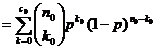
    For scenario ( n , c ) , a product is drawn from the population (lot size N ) with a defective rate p , and the probability of the defective number is

    An indicative function called scheme( n, c ) .

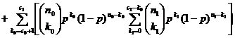
   Given the sum , is the solution of the following equation:

satisfy _

Then when n is relatively large, (that is , the integer part of nH ) is determined by the following formula:

   2 ^° Single measurement (specific data should be measured for product quality indicators) acceptance plan

    It is assumed that the quantitative indicators that measure the quality of a product follow a normal distribution and its variance is known. When (or vice versa), the product is considered qualified; when (or vice versa), the product is considered unqualified.

    Let the sample size be n , and the sample mean can be used as an indicator to judge the overall quality. Now how to choose n and L , H reasonably so that the probability of making the first or second type of error is not greater than when deciding to "accept" or "reject" the whole batch of products according to " L< " and " or " respectively a predetermined sum .

    remember

where is the normal probability integral

inverse function of . 

 

Single-type measurement acceptance plan table

 

condition	Scheme code	The program parameters are satisfied    equation set	statistical inference
			At the time , it was rejected   At that time , receiving
			At the time , it was rejected   At that time , receiving
			Reject when or     At that time , receiving

 

[ Double-piece-count sampling inspection ]   Single-type sampling acceptance scheme In order to ensure that the corresponding probability of two types of errors does not exceed , it is often necessary to draw samples with a large capacity. For the same four data , the average number of samples for double sampling is smaller than that for single sampling.

    The method of the double sampling acceptance plan is: first draw a sample with a capacity of , and set the defective product as , and compare it with the three predetermined numbers to make a judgment: if it is, then accept it in a whole batch; if it is, reject the whole batch; If , then continue to take samples with a capacity of , record the number of defectives in it , and combine the two samples. If , accept the whole batch; if , reject the whole batch. The decision is similar to the single sampling plan, to ensure that the sampling acceptance plan does not exceed the probability of rejection when the defective rate of the whole batch of products is not exceeded , and at that time , the probability of acceptance does not exceed .

The indicative function of the scheme ( ) ) is

          ; )

                     _</