Chapter 17 Error Theory and Experimental Data Processing
In scientific experiments and production practice, in order to grasp the regularity of the development of things, we always record a lot of data through various methods to observe the quantities we need. However, due to random interference from the outside world, these data actually contain random errors. Approximate data that must be appropriately processed as needed. On the one hand, it is necessary to estimate the reliability of the observed data and give a reasonable explanation ; The data ( signal ) of noise ) is analyzed and processed, and the interference is " filtered" to obtain the real required amount. The former requires the basic knowledge of error theory ( such as Gaussian error law, the calculation method of various average values, the representation of error, the law of error transfer and approximate calculation law, etc. ) , while the latter requires basic techniques for processing data ( such as interpolation, Curve fitting method, smoothing method and filtering method of experimental curve, etc. ) . This chapter describes the main elements of these methods.
§ 1 Error Theory
1. Observation error
[ True value and error ] The quantity of the observed object exists objectively and is called the true value. The value obtained for each observation is called the observed value. Assuming the true value of the observed object , the observed value is ( ), then the difference![]()
![]()
![]()
![]() ( )
( )![]()
It is called observation error, or simply error.
[ Classification and identification of errors ]
|
Classification |
cause of error |
Error identification |
|
Tie system error Difference |
(i) (ii) Changes in the surrounding environment |
(i) Observations are always biased in one direction (ii) The magnitude and sign of the error are almost the same in repeated observations
(iii) Errors can be eliminated by correction and processing |
|
follow machine error Difference |
Caused by some uncontrollable accidental factors |
The observed values are impermanent, but there are the following rules under the same precision observation ( that is, the random error obeys the normal distribution, refer to this section , 4 ) : (i) The absolute value of the error will not exceed a certain limit (ii) Errors with small absolute values appear more frequently than errors with large absolute values, and errors close to zero appear the most. (iii) The number of positive errors and negative errors with equal absolute value is almost equal (iv) the arithmetic mean of the error, which approaches zero as the number of observations increases |
|
pass lose error Difference |
Observation error or calculation error caused by rough branches and large leaves |
(i) The observations do not match the facts (ii) Careful operation can eliminate errors |
[ Accuracy and Precision of Observation ] If the systematic error of the observation is small, the accuracy of the observation is high, and more precise instruments can be used to improve the accuracy of the observation. If the random error of the observation is small, the precision of the observation is said to be high, and the number of observations can be increased to obtain the average value to improve the precision of the observation.
Errors referred to in this chapter are random errors.
2. Average value and its precision index
[ Method for finding the average value in common use ] Let it be a set of observation data of an observation object.![]()
|
name |
Definition and Notation |
Usage and Instructions |
|
Calculate technique flat all value |
|
It is the best approximation of the true value in the sense of the least squares method , and it is the most commonly used average value. |
|
simple Calculate flat all value |
set , then where is the number of groups , A is a constant , c is the group distance , is the frequency of the i -th group, and
|
|
|
Several what flat all value |
|
This method is often used when the distribution curve of the graph obtained by taking the common logarithm of a group of observations is more symmetrical ( compared with the same ) . |
|
add right flat all value |
where is the corresponding weight of the i -th observation |
When calculating the mean value of the same physical quantity observed with different methods or under different conditions, different "weights" are often given to data with different degrees of reliability. |
|
middle bit number |
The value in the middle after the observations are arranged in order of magnitude. When n is an even number, take the arithmetic mean of the middle two numbers |
It is an order statistic that can reflect the value center of a well-proportioned observation |
[ Arithmetic mean and dispersion ] The true value x of the observed object can be the arithmetic mean of n observations .![]()
![]()
Approximate instead and use dispersion
![]()
instead of errors . The dispersion is related to the error as follows![]()
![]()
![]() ( when n is quite large )
( when n is quite large )
[ precision index for mean ]
|
|
Observations with the same precision |
Observations with different precisions |
|
Observations right average value standard deviation The error of the true value x from the arithmetic mean |
1 Arithmetic mean |
Weighted average |
![]() The smaller the value is, the smaller the deviation between the mean value ( or ) of the observed value and the true value x is, and the higher the precision, that is, the higher the reliability of the mean value.
The smaller the value is, the smaller the deviation between the mean value ( or ) of the observed value and the true value x is, and the higher the precision, that is, the higher the reliability of the mean value.![]()
![]()
3. Representation of errors
Let be a set of observation data of an observation object. its arithmetic mean![]()
![]()
Error , dispersion , error of the true value from the mean .![]()
![]()
![]()
|
name and sign |
Definition and Notation |
Features |
|
[ standard error ] ( medium error or mean squared error )
|
The square root of the mean of the individual error sums of squares, i.e.
When the number of observations is large
obviously |
Does not depend on the sign of individual errors in the observations, is more sensitive to large or small errors in observations, and is a better way to express precision |
|
[ average error ]
|
the arithmetic mean of the absolute values of the dispersion
|
The advantage is that the calculation is simple, and the disadvantage is that it cannot show the coincidence of each observation. For example, the deviations in one set of observations are close to each other, while the deviations in another set of observations are large, medium and small. But the average errors obtained in these two different sets of observations may be the same. So it is more reliable only when n is large |
|
[ probability error ]
|
It is such a number that an error larger in absolute value is as likely to occur as an error smaller in absolute value, i.e.
|
After arranging the errors in order of absolute value, the median of the series is the probability error. It is difficult to find the probability error according to the arrangement, and it is more reliable only when the value of n is large. |

[ The relationship between standard error, mean error, and probability error ]
![]()
![]()
![]()
![]()
4. Gaussian Error Law
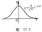
[ Gaussian Error Equation ] The distribution density function of random error is a normal distribution density function
![]()
It is called the Gaussian error equation and its graph is called the error curve
( Fig. 17.1) , where
![]() ( is the standard error )
( is the standard error )![]()
called the precision index.
The error curve is a continuous curve, when ,![]()
![]() Descending to zero.
Descending to zero.
![]() A value selected according to the actual situation as the limit, the value of x exceeding this limit is very small and is considered to be equal to zero. It is considered to be the maximum value of positive and negative errors, and the general error value is any value between and , and their probability is the value in this interval.
A value selected according to the actual situation as the limit, the value of x exceeding this limit is very small and is considered to be equal to zero. It is considered to be the maximum value of positive and negative errors, and the general error value is any value between and , and their probability is the value in this interval.![]()
![]()
![]()
![]()
![]()
![]()
![]()
![]() Positive and negative errors with equal absolute values have equal probability of occurrence.
Positive and negative errors with equal absolute values have equal probability of occurrence.
![]() An error with a small absolute value is more likely than an error with a large absolute value.
An error with a small absolute value is more likely than an error with a large absolute value.
[ Error probability table and its use ] Let denote error and denote standard error. For different t, the value of probability is as follows.![]()
![]()
![]()
Error probability table
|
Error limit |
|
|
|
|
|
probability |
0.00 |
25% |
|
|
|
Error limit |
|
|
|
|
|
probability |
|
|
|
|
The main purpose
(1) Determine the size of the probability that a given error is within a certain range, thereby judging that the error is a systematic error and a random error. For example, when the absolute value of the error is greater than ( it is only possible ) , it cannot be believed to be a random error. ![]()
![]()
(2) When using various methods to observe the same physical quantity, judge whether the obtained results are consistent with each other.
5. Errors and significant figures
[ Absolute error and relative error ] x is the true value of the observed object, and its approximate value is .![]()
|
Error name |
Definition and calculation formula |
|
absolute error maximum absolute error Relative error maximum relative error |
the smallest quantity that makes the inequality true
the smallest quantity that makes the inequality true |

[ General formula for error propagation ]
![]() Suppose a function representing m independent variables , if the maximum absolute errors of the independent variables are respectively , then the maximum absolute error and the maximum relative error of the function y are respectively
Suppose a function representing m independent variables , if the maximum absolute errors of the independent variables are respectively , then the maximum absolute error and the maximum relative error of the function y are respectively![]()
![]()
![]()
![]()
![]()
![]()

![]() Error estimates for simple operations on approximations
Error estimates for simple operations on approximations
![]()
![]()
![]() ( p is any real number )
( p is any real number )
![]()
![]() Assuming that it is regarded as a function of random variables, and the standard error and probability error are represented by and respectively, the error transfer formula is:
Assuming that it is regarded as a function of random variables, and the standard error and probability error are represented by and respectively, the error transfer formula is:![]()
![]()
![]()
![]()
[ Significant and suspicious digits ]
Any approximation can be expressed in decimal as![]()
![]()
where all are positive integers, m is the number of digits in the integer part of the approximation, or expressed as![]()
![]()
![]()
If the maximum absolute error of the approximation does not exceed half a unit from the kth digit from the left ( from the first non-zero digit on the left ) , i.e.
![]()
are called significant digits. In particular, when k=n , it is called an approximation with n significant digits.![]()
![]()
If the maximum absolute error of the approximation does not exceed one unit in the kth position from the left, i.e.![]()
![]()
are called reliable numbers. In particular, when k=n , it is called an approximation with n reliable digits.![]()
![]()
It can be seen that significant figures are more precise than reliable figures. The concept of significant digits is generally used.
If the approximation has k significant digits ( or reliable digits ) , the kth digit from the left is called the suspect digit.![]()
[ Number rule ]
![]() When recording observations, only one suspicious digit is kept.
When recording observations, only one suspicious digit is kept.
![]() Unless otherwise specified, suspicious numbers indicate an error of one unit ( or units ) on the last digit .
Unless otherwise specified, suspicious numbers indicate an error of one unit ( or units ) on the last digit .![]()
![]()
![]() When expressing precision, only one significant figure is taken in most cases, and at most two significant figures are taken.
When expressing precision, only one significant figure is taken in most cases, and at most two significant figures are taken.
![]() In data calculation, after the number of significant digits is determined, the rest of the digits should be rounded off ( by rounding ):
In data calculation, after the number of significant digits is determined, the rest of the digits should be rounded off ( by rounding ):
(i) The first digit to be rounded is less than or equal to 4 .
(ii) The first digit to be dropped is greater than 5 , or the first digit to be dropped is equal to 5 and the second digit is greater than zero, then 1 is added to the last reserved digit .
(iii) The first bit to be rounded is equal to 5 and the second bit is equal to zero, then there are two cases: 1 should be added when the last bit reserved is an odd number ;
[ Approximate calculation rule ]
![]() When adding or subtracting no more than ten approximate values, the number with more decimal places should be rounded to one more decimal place than the number with the most decimal place; the number of decimal places retained in the calculation result should be the least number of decimal places in the original approximate value. are the same.
When adding or subtracting no more than ten approximate values, the number with more decimal places should be rounded to one more decimal place than the number with the most decimal place; the number of decimal places retained in the calculation result should be the least number of decimal places in the original approximate value. are the same.
![]() When multiplying and dividing approximate values, the number of digits reserved for each factor should be 1 larger than the number of digits of the least significant number of digits, and the number of digits of the reliable digits of the resulting product ( or quotient ) should be the same as the number of digits of the least significant number of digits in the original approximate value. equal.
When multiplying and dividing approximate values, the number of digits reserved for each factor should be 1 larger than the number of digits of the least significant number of digits, and the number of digits of the reliable digits of the resulting product ( or quotient ) should be the same as the number of digits of the least significant number of digits in the original approximate value. equal.
![]() When exponentiating or rooting the approximate value, the original approximate value has several significant digits, and the calculation result can retain several digits.
When exponentiating or rooting the approximate value, the original approximate value has several significant digits, and the calculation result can retain several digits.
![]() The number of digits of the logarithm taken shall be equal to the number of significant digits of the true number.
The number of digits of the logarithm taken shall be equal to the number of significant digits of the true number.
Note that in the course of the calculation, the intermediate result should take one more digits than indicated by the above rules; but this "backup digit" is still rounded when entering the final calculation.![]()
![]() Subtracting two similar numbers or using a number close to zero as a divisor is often the cause of large relative errors in the calculation results. So if possible, the calculation procedure should be organized and avoided as much as possible. For example, the two roots of a quadratic equation in one variable are
Subtracting two similar numbers or using a number close to zero as a divisor is often the cause of large relative errors in the calculation results. So if possible, the calculation procedure should be organized and avoided as much as possible. For example, the two roots of a quadratic equation in one variable are ![]()
![]()
![]()
When b > 0 , and when, using the above formula will get wrong results. The formula should be deformed and use the formula instead![]()
![]()
![]()
![]()
Calculation.
[ Counting rules for predetermined accuracy ]
![]() If the calculation result is obtained by addition and subtraction, the original data should have one more decimal place than the result requires.
If the calculation result is obtained by addition and subtraction, the original data should have one more decimal place than the result requires.
![]() If the calculation result is obtained by multiplication, division, exponentiation, and square root, the number of significant digits of the original data should be one more than the number of digits required by the result.
If the calculation result is obtained by multiplication, division, exponentiation, and square root, the number of significant digits of the original data should be one more than the number of digits required by the result.
![]() The number of significant digits of the arithmetic mean of four or more approximations may be increased by one.
The number of significant digits of the arithmetic mean of four or more approximations may be increased by one.