§ 4 Approximate computation of real roots
Let f ( x ) be a known continuous function and ξ be the equation
f ( x ) = 0
The roots of , where the equation can be a general equation (algebraic or transcendental) . The range of the roots is given in practical problems, such as algebraic equations
f ( x )= a 0 x n + a 1 x n - 1 + L + a n - 1 x + a n =0
The range of the root ξ is
| ξ | £ 1+ max{ | a 1 | , | a 2 | , L , | a n | }![]()
Therefore, it can be assumed that the equation has only one root in the interval ( a , b ) (if there are two roots, replace one endpoint of the interval with a point where ( x )=0 ) . And from the continuity of the function, generally Said that f ( x ) is of opposite sign near the root (except when ( ξ )=0 or otherwise), so in the various approximations described below, it is assumed that f ( a ) and f ( b ) are of opposite sign .![]()
![]()
![]()
1. Qin Jiushao method *
Qin Jiushao's method is basically a method of obtaining the approximate value of the root through successive experiments. The more the number of experiments, the closer the obtained approximate value is to the true value of the root . This process is systematically continued until the number of digits of the predetermined significant figures is reached . this method .
Example equation
f ( x ) =(1)![]()
The root of to five significant digits .
Applying the Cartesian rule of symbols shows that this equation has a positive root . Since f (1) = - 11 and f (2) = 14 , this positive root is between ( 1,2) .
Now apply Qin Jiushao's method to find the approximate root of this equation . Suppose , here is the distance from 1 to the sought root . Applying the polynomial Taylor formula ( Qin Jiushao's method , see § 2, 1 ) , the equation of![]()
![]()
![]()
![]() (2)
(2)
Its formula is
![]()

Now to find the approximate value of pure decimals, since the value of the third power or quadratic power of pure decimals is smaller, the first two terms of equation (2) can be temporarily discarded to calculate 21 - 11 = 0 , that is, = 0.5238 .... The last two terms are positive, and this value appears too large . When = 0.500 , the sum of the left-hand terms of equation (2) is still positive (0.375) , and when = 0.400 , the left-hand terms of equation (2) The sum of is negative ( -2.056 ). Therefore, let , i.e. , again applying Taylor's formula for the polynomial, we get the equation for h![]()
![]()
![]()
![]()
![]()
![]()
![]()
![]() (3)
(3)
Its formula is
![]()
* Qin Jiushao, an ancient Chinese mathematician , gave an approximate value for finding the root of an algebraic equation in his book << Nine Chapters of the Book of Numbers >> ( 1247) .
method, this method is generally called Hena method in books . In fact, Hena only proposed this method in 1819 , more than Qin Jiu
Shaowan more than five hundred years ago .
![]()
Now find the approximation of the decimal h , discard the first two items, and find h = 0.08609.... Because the two positive quantities are discarded, the obtained h is too large, so set h = 0.08 , ![]() that is, apply the above method to obtain the equation of
that is, apply the above method to obtain the equation of![]()
![]()
![]() (4)
(4)
As above, from the last two terms of equation ( 4 ) , we can obtain the![]()
![]()
![]()
![]()
![]() (5)
(5)
The approximate value obtained from the last two terms = 0.0008..., since all positive quantities are discarded, the root of equation (5) is between 0.0008 and 0.00081 .![]()
![]()
Now add the approximations 0.4, 0.08, 0.004, 0.0008 of (2), (3), (4), (5), to the sum of 0.4848 , and then add to the first approximation 1 , so the equation (1) has The root is between 1.4848 and 1.48481 , taking five significant figures as 1.4848.
The Qin Jiushao method can also be used to find negative approximations . If you want to find all negative real roots of f ( x ) = 0 , you can first find the positive real roots of f ( - x ) , and then change the sign to get the negative real roots .
 2. Dichotomy
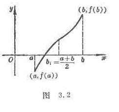
Assuming that f ( x ) is continuous on [ a, b ] , and f ( a ) f ( b )<0 (here it is assumed that f ( a )<0, f ( b )>0 ) , take the interval [ a, b ] The midpoint of , if = 0 , then the root of f ( x )=0 is ξ = . Otherwise, if > 0 , then let a 1 = a , b 1 = ; if < 0![]()
![]()
![]()
![]()
![]()
![]() , then let a 1 = , b 1 = b . Then a new interval [ a 1 , b 1 ] is formed , which contains the root ξ of f ( x ) = 0 (Fig. 3.2 ) .
, then let a 1 = , b 1 = b . Then a new interval [ a 1 , b 1 ] is formed , which contains the root ξ of f ( x ) = 0 (Fig. 3.2 ) .![]()
Then take the midpoint of [ a 1 , b 1 ] , if = 0 , then ξ = . If > 0 , then let a 2 = a 1 , b 2 = ; if <0 , then let a 2 = , b 2 = b 1 . A new interval [ a 2 , b 2 ] is thus formed , whose length is equal to that which contains the roots of the equation f ( x ) = 0 ξ . …![]()
![]()
![]()
![]()
![]()
![]()
![]()
![]() If the allowable error ε = , the interval [ a 1 , b 1 ], [ a 2 , b 2 ], [ a 3 , b 3 ], L , [ a n , b n ], n = ( [ x ] represents the integer part of x), then
If the allowable error ε = , the interval [ a 1 , b 1 ], [ a 2 , b 2 ], [ a 3 , b 3 ], L , [ a n , b n ], n = ( [ x ] represents the integer part of x), then![]()
![]()
ξ * =![]()
is the approximate root of the equation f ( x ) = 0 with an error of no more than
| ξ - ξ * | £ £![]()
![]()
The dichotomy method is the simplest and most effective method in the approximate calculation of real roots. It only requires the function to be continuous, so it has a wide range of use and is easy to implement on electronic computers . However, it cannot find multiple roots, nor can it find virtual root .
3. Iterative method
Express the equation f ( x ) = 0 in its equivalent form
x = j ( x )
or generally
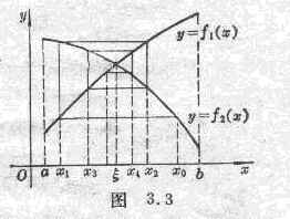
f 1 ( x ) = f 2 ( x )
where f 1 ( x ) is a function: for any real number c , it is easy to find the real root of the equation f 1 ( x ) = c with high accuracy . If for any a £ x 1 £ b , a £ x 2 £ b , the following formula holds:
Then the following iterative process is convergent .
First start from an approximate root x 0 ( x 0 can be roughly estimated by the graphical method), substitute the right side of the equation, and solve the equation
f 1 ( x ) = f 2 ( x 0 )
get the first approximate root x = x 1 , then solve the equation
f 1 ( x ) = f 2 ( x 1 )
 Obtain the second approximate root x = x 2 , L , and similarly by the nth approximate root x n , solve the equation
f 1 ( x ) = f 2 ( x n )
Get the n +1th approximate root x = x n +1 , so get a series of approximate roots with different precisions
x 0 , x 1 , x 2 , L , x n , L
It converges to the root ξ of the equation (Figure 3.3 ) .
The rate of convergence (that is, the rate of error disappearance) is comparable to a n , while
a![]()
use
![]()
 Substituting x 2 can speed up the convergence . In the formula, D x 1 = x 2 - x 1 is the first-order difference of x 1, and D 2 x 0 = D x 1 - D x 0 is the second -order difference of x 0 .
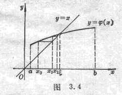
For the equation x = j ( x ) , as long as j ( x ) is continuous on [ a , b ] and q < 1 , then its root can be given by![]()
x 1 = j ( x 0 )
x 2 = j ( x 1 )
L L L L
x n + 1 = j ( x n )
to approach (Fig. 3.4 ) .
4. Newton's method
1 . General Newton's method
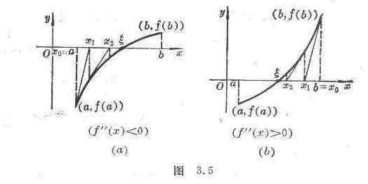
Let f ( x ) be continuous on [ a , b ] and also be continuous, and 1 0, 1 0 , f ( a ) f ( b )<0 (let f ( a )<0, f ( b )>0 ) , through the point ( a , f ( a )) (or the point ( b , f ( b ) ) ) as a tangent to the curve:![]()
![]()
![]()
![]() (or )
(or )![]()
It intersects the x -axis at x = a - (or x = b - )![]()
![]()
with iterative formula
x n + 1 = x n −![]()
and take the initial value
x 0 =
An approximation of the roots of the equation f ( x )=0 can be calculated (Fig. 3.5 ) . The error ï x – x n ï does not exceed

Generally, the initial value x 0 selected must satisfy the inequality
![]()
2 . Approximate Newton's method
If it is not easy to calculate, the difference quotient can be used instead to obtain an approximate Newton method iterative program:![]()
x n + 1 = x n![]()
3 . Sequential Compression Newton's Method
find algebraic equations with real coefficients
f ( x )= a 0 x n + a 1 x n -1 + L + a n =0
When the single real root of , after finding a real root x 0 by Newton's method , the degree of the polynomial can be reduced once, and the polynomial coefficient b k after the reduced degree is
b 0 = a 0
b k = a k + x 0 b k -1 ( k =1,2, L , n -1)
Then, using the obtained real roots as the initial approximation, use the same method to obtain the real roots of the polynomial with the reduced degree again, and then obtain all the single real roots .
4 . Newton's Method for Solving Nonlinear Systems of Equations
Assuming a nonlinear system of equations

There exists a set of approximate solutions P 0 =( x 0 , y 0 ) , and
Available iterative formulas:
x n + 1 = x n +
y n + 1 = y n +
where P n is the point ( x n , y n ) and J n is the value of Jacobian J at P n :
5. Chord intercept method (linear interpolation method)
Assuming that f ( x ) is continuous on [ a , b ] , , are invariant, and f ( a ) f ( b )<0 (it is assumed here that f ( a ) <0, f ( b )>0 ) . The line at points ( a , f ( a )) and ( b , f ( b )) is:![]()
![]()

![]() ( or )
( or )![]()
It intersects the x -axis at x = a - (or x = b - ) .![]()
![]()
( a ) When > 0 , use the iterative formula![]()
![]()
The approximate roots of the equation can be found (Fig. 3.6( a ) ) .
( b ) When < 0 , with the iterative formula![]()
![]()
The approximate roots of the equation f ( x )=0 can be found (Fig. 3.6( b ) ) .
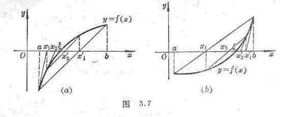
6. Combined method (Newton's method and chord cut method are used in combination)
Assume that f ( x ) is continuous on [ a , b ] , , are invariant, and f ( a ) f ( b )<0 (here it is assumed that f ( a )<0, f ( b ) >0 .![]()
![]()
( a ) When f ( a ) has the same sign (Fig. 3.7( a ) ), use the iterative formula![]()
x1 = a _![]()
![]() = b
= b![]()
x2 = x1 _ _![]()
![]() =
=![]()
![]()
L L L L L L L
x n = x n -1![]()
![]() =
=![]()
![]()
The approximate roots of the equation f ( x )=0 can be found .
( b ) When f ( a ) has an opposite sign (Fig. 3.7( b ) ), using the iterative formula![]()
x1 = a _![]()
![]() = b
= b![]()
x2 = x1 _ _![]()
![]() =
=![]()
![]()
L L L L L L L L
x n = x n -1![]()
![]() =
=![]()
![]()
The approximate roots of the equation f ( x )=0 can be found .
error or .![]()
![]()
7. Parabolic method (Mueller method)
Find the nth degree equation with real coefficients
f ( x )= x n + a 1 x n -1 + L + a n =0 (1)
approximate root of .
A root x = r of f ( x )=0 can be found first , then
f ( x )=( x - r ) g ( x )
=( x - r )( x n - 1 + b 1 x n - 2 + L + b n - 1 )
In the formula, g ( x ) is a polynomial of degree n - 1 , and then find the roots of g ( x ) , and so on, you can find all real roots of f ( x )=0 .
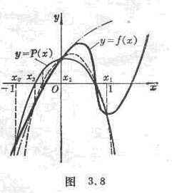 First select three points on the x -axis: x 0 , x 1 , x 2 , through the three points on the curve y = f ( x ) : ( x 0 , f ( x 0 )), ( x 1 , f ( x 1 ) ), ( x 2 , f ( x 2 )) as a parabola y = P ( x ) (i.e. Lagrangian interpolation polynomial, see Chapter 17, § 2 , 3), the parabola and xThe axis has two points of intersection, take the point closer to x 2 as x 3 ; then three points ( x 1 , f ( x 1 )), ( x 2 , f ( x 2 )), ( x 3 , f ( x 3 )) to draw a parabola ( dotted line in Figure 3.8 ), which has two intersection points with the x -axis, take the point closer to x 3 as x 4 L , and make points x i -2 , x i - according to this method 1 , x i , after three o'clock (x i -2 , f ( x i -2 )), ( x i -1 , f ( x i -1 )), ( x i , f ( x i )) as a parabola has two intersections with the x -axis, Take the point closer to xi as xi +1 , and so on .
For a predetermined allowable error e , when the iterative process proceeds to
ï x i + 1 - x i ï < e
, take x i +1 as an approximate root of f ( x )=0 .
The resulting sequence is convergent . The limit is the root of the equation f ( x )=0 .![]()
The iterative steps are as follows:
( 1 ) According to experience, the above formula ( 1 ) is desirable
x 0 =-1, x 1 =1, x 2 =0
as the initial value, so
f ( x 0 )=(-1) n +(-1) n - 1 a 1 + L - a n - 1 + a n
f ( x 1 )=1+ a 1 + L + a n
f ( x 2 ) = a n
or with an approximation around x = 0
f ( x 0 ) » a n − 2 − a n − 1 + a n
f ( x 1 ) » a n − 2 + a n − 1 + a n
f ( x 2 ) = a n
( 2 ) set
l i = , d i =1+ l i =![]()
![]()
g i = f ( x i - 2 ) l i 2 - f ( x i -1 ) l i d i + f ( x i ) l i
h i = f ( x i -2 ) l i 2 - f ( x i -1 ) d i 2 + f ( x i )( l i + d i )
From this , l i , d i , g i , hi are calculated from x i -2 , x i -1 , xi , and l i +1 is calculated according to the following formula
l i +1 =
( h i >0 , the radical takes the positive sign; h i <0 , the radical takes the negative sign)
When f ( x i -2 ) = f ( x i -1 ) = f ( x i ) , take l i +1 =1.
( 3 ) According to the formula
x i + 1 = l i +1 ( x i - x i -1 )+ x i
Calculate x i +1
8. Lin Shizhen - Zhao Fangxiong's method (split factor method)
Since it is easy to solve quadratic equations, in finding real coefficient algebraic equations
f ( x )= x n + a 1 x n - 1 + L + a n - 1 x + a n =0
If you find a quadratic factor of f ( x ) when you find the complex roots of , it is equivalent to finding a pair of complex roots of the equation .
Let an approximate quadratic factor (chosen arbitrarily) of f ( x ) be
w ( x ) = x 2 + px + q
It can be refined in the following ways:
( 1 ) Divide f ( x ) by w ( x ) to obtain the quotient Q ( x ) and the remainder R ( x ) , namely
f ( x )= w ( x ) Q ( x )+ R ( x )
=( x 2 + px + q )( x n - 2 + b 1 x n - 3 + L + b n - 3 x + b n - 2 )+( r 1 t + r 2 )
The coefficients of the quotient and remainder in the formula can be calculated by the following recursive formula:
b k = a k - pb k -1 - qb k -2 , k =1,2, L , n
b -1 = 0, b 0 =1
r 1 = b n -1 = a n -1 - pb n -2 - qb n -3
r 2 = b n + pb n -1 = a n - qb n -2
( 2 ) Divide xQ ( x ) by w ( x ) to get the remainder
R [ 1] ( x ) = R 11 x + R 21`
where R 11 , R 21 are calculated by the following recursive formula:
c k = b n - pc k -1 - qc k -2 , k =1,2, L , n -3
c -1 = 0, c 0 =1
R 11 = b n -2 - pc n -3 - qc n -4
R 21 =- qc n -3
( 3 ) Divide Q ( x ) by w ( x ) to get the remainder
R [ 2] ( x ) = R 12 x + R 22`
where R 12 , R 22 are calculated from the following formula:
R 12 = b n -3 - pc n -4 - qc n -5
R 21 = b n -2 - qc n -4
( 4 ) Solve binary linear equation system
get u , .![]()
( 5 ) The corrected quadratic formula is
w [1] ( x )= x 2 +( p + u ) x +( q +)![]()
If it is not accurate enough, repeat steps ( 1 ) to ( 5 ) to correct it until it is accurate enough .
The Lin Shichen - Zhao Fangxiong method for finding complex roots of algebraic equations with real coefficients has the advantage of avoiding complex operations, but the disadvantage is that the program is more complicated .
9. Descending method
Transcendental equations for arbitrary real coefficients
 (1)
(1)
Define the objective function
F ( x 1 , x 2 , L , x n )=![]()
If F ( x 1 , x 2 , L , x n ) < e ( e is a suitably small positive number given with a certain precision), then x 1 , x 2 , L , x n is considered to be a system of equations ( 1 ) solution .
The specific calculation steps are as follows:
( 1 ) Take any set of initial values x 1 (0) , x 2 (0) , L , x n (0) (all not zero), suppose that the mth step has been calculated according to the following process to obtain a set of values : x 1 ( m ) , x 2 ( m ) , L , x n ( m )
( 2 ) Calculation
F m = F ( x 1 ( m ) , x 2 ( m ) , L , x n ( m ) )
( 3 ) If F m < e , then x 1 ( m ) , x 2 ( m ) , L , and x n ( m ) are the solution to be solved, otherwise calculate n partial derivatives:
![]() [ F ( x 1 ( m ) , x 2 ( m ) , L , x i ( m ) + H i , L , x n ( m ) ) - F ( x 1 ( m ) , x 2 ( m ) , L , x n ( m ) ) ]
[ F ( x 1 ( m ) , x 2 ( m ) , L , x i ( m ) + H i , L , x n ( m ) ) - F ( x 1 ( m ) , x 2 ( m ) , L , x n ( m ) ) ]
H i = w x i ( m ) i =1,2, L , n
( 4 ) Calculation
x i ( m +1) = x i ( m ) , i =1,2, L , n![]()
in the formula
Get a set of { x i ( m +1) } , and repeat the calculation of ( 2 ), ( 3 ) , ( 4 ) .