Chapter 5 Differential Calculus
The research method of calculus is the limit method, and the research object is the function (especially the elementary function). The main content of calculus is the differential method , the integral method and their applications . Applications (theory of implicit functions , expansion of functions into power series , extrema of functions, and graphing), also introduces the concept and properties of continuity of functions, as well as number series , double series , function series, and infinity Convergence concepts and discriminant methods of products . Taking into account the uniform continuity of functions, uniform convergence of function term series, and the importance of the concepts of function differentiability in theory and practice, this chapter focuses on these concepts and introduces Examples are given to illustrate the essence of these concepts . In addition, the power series expansions of some common elementary functions are collected and listed for reference .
§ 1
Limits of sequences and functions
The limit of
the sequence
1 . basic concept
[ Finite limit ] Suppose that for any small ε > 0, there exists a positive integer N = N ( ε ) such that for all n > N , the inequality
| x n - a | < ε ( a is a finite number )
If established, it is called the sequence x 1 , x 2 , ( referred to as { x n }) with a as the limit ( or the sequence converges to a ) , denoted as![]()
![]()
Otherwise the sequence is called divergent .
[ Infinite Limit ] Suppose that for any large E > 0 , there exists a positive integer N = N ( E ) such that for all n > N , the inequality
| x n | > E
If it is established, the limit of the sequence x 1 , x 2 , is called ∞ (or the sequence diverges at ∞ ), denoted as![]()
![]()
[ Partial limit ( cluster point )] In the elements of the known sequence x 1 , x 2 , keep the original order and select an infinite number of elements arbitrarily from left to right, such as![]()
![]()
Such a sequence is called a subsequence of a known sequence . If
![]()
The number ξ (or the symbol ∞ ) is called a partial limit ( or focal point ) of the known sequence { x n } .
Any sequence { x n }, whether bounded or unbounded, has some limits .
[ Upper limit and lower limit ] The largest partial limit (finite or infinite) of the sequence { x n } is called the upper limit of the sequence { x n } , denoted as
![]()
And its smallest partial limit (finite or infinite) is called the lower limit of the sequence { x n } , denoted by
![]()
Therefore, a sequence { x n } does not converge if two subsequences do not converge to the same limit . If
![]() , that is, the sequence { x n } converges to a , then any subsequence { } of { x n } converges to a .
, that is, the sequence { x n } converges to a , then any subsequence { } of { x n } converges to a .![]()
2 . The Discriminant Method of Existence of Sequence Limit
[ Cauchy criterion ] The necessary and sufficient condition for the existence of the limit of the sequence { x n } is: for any given ε > 0 , there exists a positive integer N = N ( ε ) such that when n > N , the inequality
| | < ε![]()
This holds for all positive integers p > 0 .
[ The upper and lower limits are equal ] The necessary and sufficient conditions for the existence of the limit (finite or infinite) of the sequence { x n } are:
![]() =
=![]()
[ Monotone Bounded ] A monotone bounded sequence must have a limit .
If { x n } is an increasing sequence and x n ≤ M ( n =1,2,…) , exists and does not exceed M .![]()
If { x n } is a descending sequence, and x n ≥ M ( n = 1,2,…) , exists and is not less than M .![]()
[ with bounded variation ] * a sequence of bounded variation ( ie there is a positive number c such that | | + | | +![]()
![]()
![]() | < c , n = 2, 3, there must be a limit .
| < c , n = 2, 3, there must be a limit .![]()
[ Sequence comparison ] If the sequence { x n } satisfies the condition y n ≤ x n ≤ z n , and == c , then![]()
![]()
![]() = c
= c
[ Stuyz's theorem ] For a sequence , if (i ) n ≥ n 0 ( n 0 is a natural number ) , y n +1 > y n , (ii) =+ ∞ , (iii) = l ( a finite number or ) , then![]()
![]()
![]()
![]()
![]()
![]()
![]()
![]() = = l
= = l![]()
![]()
[ Weighted Average Sequence ] Let w nk ≥ 0 ( k = 1,2, n ; n =1,2 ), =1, for a fixed k , w nk =0. If x n = a , then = a ![]()
![]()
![]()
![]()
![]()
![]()
![]()
3 . Basic formula for sequence limit
If x n , y n exist, then![]()
![]()
![]() ( x n y n ) = x n y n
( x n y n ) = x n y n![]()
![]()
![]()
![]()
![]()
* For functions with bounded variation is defined as follows: Assuming that f ( x ) is finite on [ a , b ] , make a bisector on [ a , b ] a = x 0 < x 1 <…
<x n- 1 <x n = b, as a sum , the supremum of V is called the total variation of f ( x ) over [ a , b ] , denoted as .![]()
![]()
If <+ , then f ( x ) is said to have bounded variation in [ a , b ] .![]()
![]()
![]() ( x n · y n ) = x n · y n
( x n · y n ) = x n · y n![]()
![]()
![]()
![]() = ( when y n ≠ 0 ) _
= ( when y n ≠ 0 ) _![]()
![]()
![]() x n y n (when y n )
x n y n (when y n )![]()
![]()
4 . Limits of Common Sequences
![]()
![]() = = = e =
= = = e =![]()
![]()
![]()
![]()
![]()
![]()
![]() = e
= e
![]() (1+1+ )= e
(1+1+ )= e![]()
![]() n ( -1) = ( a > 0)
n ( -1) = ( a > 0)![]()
![]()
![]()
![]() =1
( a > 0)
=1
( a > 0)
![]()
![]() =1
=1
![]()
![]() = ∞
= ∞
![]() [(1+ )- ]= γ
[(1+ )- ]= γ![]()
![]()
where γ = is Euler's constant .![]()
The limit of the function
1. basic concept
[ Bilateral limit ( the limit of a function at a certain point )] If for any small ε > 0 , there exists a positive number δ = δ ( ε ) such that for all values x that satisfy the inequality 0 < | x - a | ≤ ≤ ,| A - f ( x )| < ε are all established, then the number A is called the limit of the function f ( x ) at point a , denoted as
![]() = A
= A
[ One -sided limit ( left limit and right limit )] If for any small ε > 0 , there is a positive number , so that for all values x that satisfy the inequality , it is true, then the number A ′ is called a function f ( x ) At the left limit of point a , denoted as![]()
![]()
![]()
![]()
If there is a positive number for any small value, so that it holds for all the values x that satisfy the inequality , then the number A ″ is called the right limit of the function f ( x ) at point a , and is written as![]()
![]()
![]()
![]()
![]() f ( x )= f ( a +0)= A ″
f ( x )= f ( a +0)= A ″
[ Infinite Limit ] If for any large positive number M , there is a positive number , so that for all values x that satisfy the inequality , there is always![]()
![]()
| f ( x )| > M
Then the limit of the function f ( x ) at point a is ∞ , denoted as
![]() =
=![]()
[ local limit ] If there is an equation for some sequence x n → a
![]() = B
= B
Then the number B ( or the symbol ∞ ) is said to be the local limit ( finite or infinite ) of the function f ( x ) at point a .
[ Upper limit and lower limit ] The smallest and largest in the local limit are respectively used
![]() and
and![]()
to represent, they are called the lower limit and upper limit of the function f ( x ) at point a , respectively .
2. The Discriminant Method of Existence of Function Limit
[ Cauchy Criterion ] The necessary and sufficient condition for the existence of the limit of the function f ( x ) at point a is: for any small value , there exists a number > 0 , such that it satisfies![]()
![]()
![]() and
and ![]()
Any two points x ′ and x ″ ( x ′ and x ″ are in the domain of the function f ( x ) ) , have
![]()
[ Limit on any convergent sequence ] The necessary and sufficient condition for the existence of the limit of the function f ( x ) at point a is: for any sequence { x n }( n =1, ) that converges to a , there are![]()
![]() = A
= A
Then the limit of the function f ( x ) at point a is A .
[ The left and right limits are equal , the upper and lower limits are equal ] The sufficient and necessary conditions for the existence of the limit of the function f ( x ) at point a are: the left limit is equal to the right limit, or the upper limit is equal to the lower limit, that is
f ( a +0) = f ( 0)![]()
or
![]() =
=![]()
[ Monotone bounded ] A monotone bounded function must have a limit .
If f ( x ) is a monotonically increasing function in the interval ( a , b ) , and in the interval ( a , b ) , then f ( x ) must exist and not exceed M .![]()
![]()
If f ( x ) is a monotonically decreasing function in the interval ( a , b ) , and in the interval ( a , b ) , then f ( x ) must exist and be not less than M .![]()
![]()
[ Function comparison ] If , and f 1 ( x )= f 2 ( x )= A , then![]()
![]()
![]()
![]() f ( x ) = A
f ( x ) = A
3. Basic formula for the limit of a function
Let f ( x ), g ( x ) exist, then![]()
![]()
![]() ( f ( x ) g ( x )) = f ( x ) g ( x )
( f ( x ) g ( x )) = f ( x ) g ( x )![]()
![]()
![]()
![]()
![]() ( f ( x ) g ( x ) ) = f ( x ) g ( x )
( f ( x ) g ( x ) ) = f ( x ) g ( x )![]()
![]()
![]()
![]() = (when g ( x ) ≠ 0 )
= (when g ( x ) ≠ 0 )
![]()
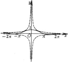
4. Limits of some important functions
|
Functions and Graphics |
Limits and Features |
|
|
The curve is symmetrical about the y -axis limit
[ Note ] |
|
|
The curve is symmetrical about the y -axis limit |
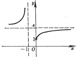
|
|
Asymptotes y=e and x = - 1 limit
[ Note ] |
|
|
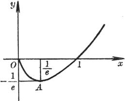
minimum point limit [ Note ] |
|
|
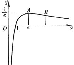
Maximum point A ( e ,
) Inflection point B ( , ) Asymptotes y = 0 and x = 0 limit =0
[ Note ] |
|
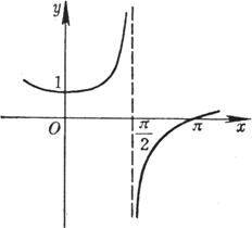
|
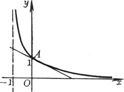
Asymptotes y = 0 and x = - 1 limit
|
|
|
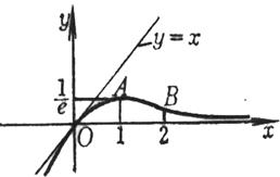
The intersection with the y - axis is O (0,0), the slope of the tangent at this point is 1
Maximum point A (1, ) Inflection point B (2, ) Asymptote y = 0 limit
[ Note ] |
|
|
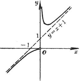
The curve consists of two Discontinuity point x = 0 Asymptote y = x +1 limit
|
|
|
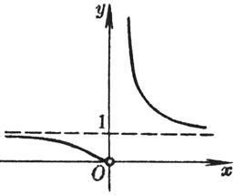
Discontinuity point x = 0 Asymptotes y = 1 and x = 0 limit
|
5 . The method of determining the value of an infinitive - Lobida's Law
![]()
Lobida's Law is a law used to calculate the limits of seven infinitives such as , , , , 0 , 0 , etc. *.![]()
![]()
![]()
![]()
![]()
![]()
![]()
* In addition to applying Lobida's law, the calculation of the limit can also be expanded by the Taylor series of the function ( § 3.8 ) , which expands the infinitive
Open to find the limit .
[ Lobida's first rule ( ) ] Let ( i ) the functions f ( x ) and g ( x ) be defined in the interval ( a , b ) , ( ii ) f ( x )=0, g ( x ) =0,( iii ) in the interval ( a , b ) there is a finite derivative sum , and ≠ 0 , ( iv ) there is a limit ( finite or infinite )![]()
![]()
![]()
![]()
![]()
![]()
![]()
![]() = K
= K
then = = K ![]()
![]()
![]()
![]()
If it is an infinitive again, the above method can be used to find the limit .![]()
![]()
![]()
[ Lobida's second law ( ) ] Let ( i ) the functions f ( x ) and g ( x ) be defined in the interval ( a , b ) , ( ii ) f ( x ) = , g ( x ) = , ( iii ) in the interval ( a , b ) there is a finite derivative sum , and ≠ 0 , ( iv ) there is a limit (finite or infinite)![]()
![]()
![]()
![]()
![]()
![]()
![]()
![]()
![]()
![]() = K
= K
then = = K ![]()
![]()
![]()
![]()
If it is an infinitive form again, the above method can be used to find the limit.![]()
![]()
![]()
[ other type infinitives ( , , , 0 , 0 ) ]![]()
![]()
![]()
![]()
![]()
1 ° to the infinitive of the form, you can first turn it into a form or form, and then apply Lobida's law. Assume ![]()
![]()
![]()
![]() f ( x )=0, g ( x )=
f ( x )=0, g ( x )=![]()
![]()
If you want to calculate f ( x ) · g ( x ), then you can do the deformation![]()
f ( x ) g ( x ) = =![]()
![]()
Among them, the second form is a form infinitive, and the third form is a form infinitive .![]()
![]()
![]()
The infinitive of the 2 ° type can also become a type or type, if you want to calculate [ f ( x ) - g ( x )], here ![]()
![]()
![]()
![]()
![]() f ( x )=+ , g ( x )=+
f ( x )=+ , g ( x )=+![]()
![]()
![]()
Then the following transformations can be made to turn it into an infinitive:![]()
f ( x ) - g ( x )=
3 ° For infinitives of type 0 and 0 , these expressions can be taken logarithmic in advance . ![]()
![]()
![]()
设y=[f(x)]g(x),则![]() y=g(x)
y=g(x)![]() f(x).
f(x). ![]() y的极限就是
y的极限就是![]() 型的不定式.假如用上述任一方法能求出
型的不定式.假如用上述任一方法能求出![]()
![]() y,比如它等于k(或+
y,比如它等于k(或+![]() ,或-
,或-![]() ),那末
),那末![]() y就等于ek(或
y就等于ek(或![]() ,或0).
,或0).
6.函数无穷小和无穷大的阶(符号O*,o,O,~)
If = 0, the function is called an infinitesimal at that time ; if = , then the function is called an infinitesimal at that time .![]()
![]()
![]()
![]()
![]()
![]()
![]()
![]()
![]()
Symbols O * , o , O , ~
|
symbol |
Definition |
meaning |
|
When x → a , = ( ) |
(0< < ) |
represents the function and in the process of x → a , in a narrow sense, are infinitesimals or infinites of the same order . |
|
= ( ) when x → 0 _ ( n > 0) |
(0< < ) |
is said to be infinitesimal of order n for infinitesimal x , for example, when x → 0 , |
|
When x →∞ , = ( ) ( n > 0) |
(0< < ) |
is said to be infinity of order n for infinity x . For example, when x → ,
|
|
= o ( ) when x → a _ |
|
Indicates that as x → a , the function is infinitesimal of higher order for functions, or the function is infinitesimal of lower order for functions . For example, when x → 0 , |
|
= O ( ) when x → a _ |
(0 ≤ < ) |
When x → a , the infinitesimal order of the function ( in the broad sense ) is not lower than the order of a positive function infinitesimal ( or the order of function infinity is not higher than the order of function infinity ). For example, when x → , |
|
When x → a , ~ |
|
The function is said to be equivalent to when x → a . For example, when x → 0 , there is ~ x , tan x ~ x , ~ ( a >0 ) ,
|
Third, the continuity of the function
1 . Continuity of univariate functions
[ The function is continuous at one point ] The continuity of the function f ( x ) at the point x 0 can be defined in the following ways:
Definition 1 If f ( x ) = f ( x 0 ) = f ( ), then f ( x ) is continuous at point x 0 .![]()
![]()
Definition 2 If f ( x 0 + 0 ) = f ( ) = f ( x 0 ), then f ( x ) is continuous at point x 0 .![]()
Definition 3 (Cauchy) If for any small ε > 0 , there is a positive number δ > 0 such that when | | < δ , there is always ![]()
| f ( x ) - f ( x 0 )| < ε
Then f ( x ) is continuous at point x0 .
Definition 4 When the change Δx of the independent variable is infinitesimal, the change Δy of the function is also infinitesimal , or it can be written as
![]()
![]() = [ f ( x 0 + Δ x ) ( x 0 )]=0
= [ f ( x 0 + Δ x ) ( x 0 )]=0![]()
![]()
Then f ( x ) is continuous at point x0 .
Definition 5 (Heine) if constant for any sequence { x n } limited by x 0
![]() f ( x n ) = f ( x 0 )
f ( x n ) = f ( x 0 )
Then f ( x ) is continuous at point x0 .
Definition 6 (Bell) Let f ( x ) be defined on [ a , b ] , x 0 is a point in [ a , b ] , denoted as a small closed interval containing x 0 ( it is contained in [ a , b ] ) , respectively record the upper and lower bounds , called the amplitude of f ( x ) on the upper . When the interval is infinitely contracted to a point, the limit exists, which are respectively recorded as .![]()
![]()
![]()
![]()
![]()
![]()
![]()
![]()
if
![]() =0
=0
Then f ( x ) is continuous at point x0 .
The above definitions are all equivalent .
[ The function is continuous on one side at a point ]
If f ( x ) = f ( x 0 +0) = f ( x 0 ), then f ( x ) is said to be continuous to the right of point x 0 .![]()
If f ( x ) = f ( x 0 - 0) = f ( x 0 ), then f ( x ) is said to be continuous to the left of point x 0 .![]()
[ Function is continuous on an interval ] If the function f ( x ) is defined on the interval [ a , b ] , and it is continuous at any point x on this interval , then f ( x ) is said to be continuous on the interval [ a , b ] ( The open interval ( a , b ) can be defined in the same way) .
It should be pointed out here that since the function f ( x ) may not exist at all outside the interval [ a , b ] , the continuity of the function at the endpoints should be understood as one-sided continuity: right continuous at point a , left continuous at point b continuous .
[ Discontinuous (or discontinuous) point of a function ] From the definition of a function being continuous at one point, there are only two types of discontinuous points:
1° Both limits f ( a ) and f ( a +0) exist, and the equation f ( a ) = f ( a ) = f ( a +0) does not hold, this discontinuity is called the first type discontinuity point .![]()
![]()
At least one of the two limits above 2° does not exist, and such discontinuities are called discontinuities of the second kind .
[ Operation of continuous functions ]
The algebraic sum of a 1° continuous function is a continuous function .
The product of a 2° finite number of continuous functions is a continuous function .
3° The quotient of two continuous functions (when the denominator is not equal to zero) is a continuous function .
4° Continuity of composite functions: If the function f ( x ) is continuous on the interval [ a , b ] , and the function ( y ) is also continuous on a certain interval, and the interval contains the function y = f ( x ) in All values taken on the interval [ a , b ] , then the composite function [ f ( x )] is also continuous on the interval [ a , b ] .![]()
![]()
[ Properties of Continuous Functions ]
1 ° If the function f ( x ) is continuous at point x=a , and f ( a ) > 0 ( or f ( a ) < 0) , then f ( x ) is in a certain neighborhood of point a (that is, the open interval ( All points within a - , a + ), > 0 arbitrarily small) have f ( x ) > 0 ( or f ( x ) < 0). ![]()
![]()
![]()
The boundedness theorem of 2 ° functions A continuous function f ( x ) on a closed interval [ a , b ] must be bounded on this interval .
3 ° Maximum-Minimum Theorem If the function f ( x ) is continuous in the closed interval [ a , b ] , then there is at least one point x in this interval , so that the corresponding f ( x ) value is maximum, and there is also at least one point x , Minimize the value of f ( x ) .
4 ° Intermediate Value Theorem If the function f ( x ) is continuous on the closed interval [ a , b ] , f ( a ) = A , f ( b ) = B , and let K be any value between A , B , Then there is at least one point x in this interval such that the value of f ( x ) is equal to K. In particular , if A and B are different signs, then in this interval there is at least one point x that makes the value of f ( x ) equal to zero .
5 ° Continuity of inverse functions If the function y = f ( x ) is increasing and continuous on the interval [ a , b ] , and f ( a ) = , f ( b ) = , then the inverse function x = ( y ) is on the interval [ a , b ] [ , ] is also continuous . ![]()
![]()
![]()
![]()
![]()
6 ° Continuity of functions specified in parameters If the functions ( t ) and ( t ) are defined and continuous in the interval ( , ) , and the function ( t ) is strictly monotonic in this interval, then the system of equations ![]()
![]()
![]()
![]()
![]()
x = ( t ), y = ( t )![]()
![]()
Define y as a single-valued continuous function of x in the interval ( a , b ) :
y = [ -1 ( x )]![]()
![]()
where a = and b = .![]()
![]()
[ Continuity of elementary functions ]
Generally speaking, basic elementary functions , , , , , ,![]()
![]()
![]()
![]()
![]()
![]()
![]() , , and their resulting functions after a finite number of arithmetic operations and compound function operations are continuous at all points that make them meaningful .
, , and their resulting functions after a finite number of arithmetic operations and compound function operations are continuous at all points that make them meaningful .![]()
![]()
[ The bound of the set of real numbers ]
1 ° A bounded set has a certain set of real numbers E , if there is a number M , such that all the numbers in the set E, the set E is said to be upper bound . Similarly, if there is a number m , such that all the numbers in the set E are upper bound. number , the set is said to be lower bound . A set that has both an upper and lower bound is called a bounded set . ![]()
![]()
2 ° The supremum and infimum of the set of real numbers
Definition 1 If there is a number such that there is no greater than number in the set E of real numbers, but no matter how small > 0 , there is always a number greater than - in E , then it is called the supremum of the set E , denoted as sup E. If there is a number such that the set ![]()
![]()
![]()
![]()
![]()
![]()
![]()
There is no less than number in E , but no matter how small > 0 , there is always a number less than + ε in E , then α is called the infimum of the set E , denoted as inf E .![]()
![]()
![]()
Definition 2 The smallest upper bound of a set of real numbers is called its supremum, and the largest lower bound is called its infimum .
The above two definitions are equivalent .
3 ° Existence Theorem A set with an upper bound must have a unique supremum, and a set with a lower bound must have a unique infimum .
[ Consistent continuity of functions ]
Consistent Continuity Definition of 1 ° Function Let the function f ( x ) be defined on a certain interval X ( closed or not, finite or infinite), if for any given ε > 0 , there is a Only with respect to δ = δ ( ε ) > 0 , such that for any two points x 1 and x 2 on the interval X , as long as ![]()
| x 2 - x 1 | < δ
there are inequalities
| f ( x 2 ) ( x 1 ) | < ε![]()
If it holds, then the function f ( x ) is said to be uniformly continuous on the interval X.
Note that the continuity of the function at every point on the interval does not necessarily infer its consistent continuity on the interval .
Example function f ( x ) = every point is continuous in the open interval (0,1) , but not uniformly continuous in (0,1) . In fact, for any small δ 0 , let x 1 = δ , x 2 = 2 δ , then | x 2 - x 1 |= δ , and | f ( x 2 ) - f ( x 1 )|= . At this time, | x 2 - x 1 | can be arbitrarily small, but ![]()
![]()
![]() | f ( x 2 ) -f ( x 1 )| can be arbitrarily large, so it is not consistent .
| f ( x 2 ) -f ( x 1 )| can be arbitrarily large, so it is not consistent .
It is worth noting that there is no longer a similar situation on the closed interval [ a ,b] , which is the following
2 ° Cantor's Theorem If a function f ( x ) is continuous on a closed interval [ a , b ] , then it is also uniformly continuous on this interval .
3 ° set
![]() = sup | f ( x 1 ) - f ( x 2 )|
= sup | f ( x 1 ) - f ( x 2 )|
where x 1 and x 2 are any two points in ( a , b ) suitable for | x 2 - x 1 | , and the function ω f is called the continuous modulus of the function f ( x ) .![]()
The necessary and sufficient condition for the function f ( x ) to be uniformly continuous in the interval ( a , b ) is
![]()
2 . Continuity of multivariate functions
[ Limits of multivariable functions ]
Let the function u = f ( P ) = f ( x 1 , , x n ) be defined in the region D , and P 0 ( ) is a point in D. For any small ε > 0 , all There exists δ = δ ( ε , P 0 ) > 0 such that as long as P D and 0 < ρ ( P , P 0![]()
![]()
![]() ) < δ (where ρ ( P , P 0 ) is the distance between the points P and P 0 ), both
) < δ (where ρ ( P , P 0 ) is the distance between the points P and P 0 ), both
| f ( P ) - A | < ε
Then the number A is called the limit of the function f ( P ) at point P 0 , denoted as
![]() or
or![]()
[ n -fold limit and cumulative limit ] The limit of
the above function f ( x 1 , , x n ) is obtained when all the independent variables of the function tend to their respective limits at the same time, which is called the n -fold limit (at n = 2 , respectively called double limit, triple limit , etc.) . In addition, there is also a limit, which is obtained by each independent variable tending to the limit one after another in a certain order, which is called the accumulated limit . For example, for For a binary function f ( x , y ) , the double limit is , the two accumulative limits are (first let the independent variable x tend to a , then let the independent variable y tend to b ) and (first let the independent variable y tend to be b , then let the independent variable![]()
![]()
![]()
![]()
![]()
![]()
![]()
![]()
![]() x tends to a ), the three are not necessarily equal .
x tends to a ), the three are not necessarily equal .
Theorem if ( i ) double limit
A =![]()
exists (finite or infinite), ( ii ) for any y within D , the (finite) singlet limit on x
![]() =
=![]()
![]()
exists, the limit is
![]()
![]() =
=![]()
![]()
![]()
must exist and is equal to the double limit .
Similar results are obtained for the second tired limit .![]()
![]()
![]()
[ Continuity of multivariate functions ]
Definition 1 If = = , then it is continuous at point P 0 .
![]()
![]()
![]()
![]()
![]()
Definition 2 If for any small ε > 0 , there is a positive number δ > 0 , so that when 0 < ρ ( P , P 0 ) < δ , there is always a positive number δ > 0
| f ( P ) - f ( P 0 )| < ε
Then it is continuous at point P 0 .![]()
Definition 3 When the change of the independent variable Δ x i ( i = 1 , 2 , … , n ) is infinitesimal, the change of the function is also infinitesimal, or written as
![]()
![]()
where f ( x 1 , x 2 ,…, x n ) is continuous at point ( ) .![]()
![]()
If the function is continuous at every point on the region D , then the function is said to be continuous on the region D.![]()
![]()
[ Consistent Continuity of Multivariable Functions ] Assuming that the
function is defined in a certain region D (finite or infinite), for any given ε > 0 , there exists a δ = δ ( ε ) that is only related to ε > 0 , so that for any two points P 1 and P on area D , as long as![]()
![]()
ρ ( P 1 , P ) < δ![]()
there are inequalities
| f ( P 1 ) - f ( P )| < ε![]()
If it holds, the function is said to be uniformly continuous on the region D.![]()
[ Properties of Multivariate Continuous Functions ]
A function 1 ° continuous on a bounded closed region D must be bounded on D.
2 ° A function that is continuous on a bounded closed region D must reach a maximum and a minimum on D.
3 ° A function that is continuous at every point on a bounded closed region D must be uniformly continuous on D.