10. Application of Differentiation ( I ) —Extreme Value of Function
1 . extremum of a univariate function
[ extreme (maximum or minimum) ] if the function f ( x ) is defined in the two-sided neighborhood of point x 0 , and for everything within a neighborhood 0 < | x - x 0 | < δ At point x , the following inequality holds:
f ( x )< f ( x 0 )(or f ( x )> f ( x 0 ))
Then the function f ( x ) is said to have a maximum (or minimum ) at the point x0 .
[ Necessary conditions for the existence of extreme values ] Assume that the function f ( x ) has a finite derivative in the interval ( a , b ) . If the function has an extreme value at the point x 0 ( ∈ ( a , b )) , there must be
![]() =0 (1)
=0 (1)
Therefore, the extreme value of the differentiable function can only be reached at the point where the formula (1) is established, and this point is called the stable point .
[ Sufficient conditions for the existence of extreme values ]
First Law If the function f ( x ) satisfies the condition: ( i ) is defined and continuous in some neighborhood of point x 0 | x - x 0 | < δ , and at point x 0 , = 0 or does not exist, ( ii ) has finite derivatives in the range 0 < | x - x 0 | < δ , ( iii ) has fixed signs to the left and right of point x 0 , then the function f ( x ) has no extremum at point x 0 See the table below: ![]()
![]()
![]()
|
x |
x < x 0 |
x 0 |
x> x 0 |
f ( x ) |
|
|
+ — + — |
0 |
— + + — |
maximum minimum rise decline |
Second Law if the function f ( x ) has a second derivative and at point x0 the following holds: ![]()
![]() =0 and ≠ 0
=0 and ≠ 0![]()
Then the function f ( x ) has an extreme value at this point, when < 0 , there is a maximum value; when > 0 , there is a minimum value . ![]()
![]()
Third Law Let the function f ( x ) have a derivative in some neighborhood | x - x 0 | < δ , , and ![]()
![]()
![]() =0 ( k =1 ,
=0 ( k =1 ,![]() )
)
![]() ≠ 0
≠ 0
If n is an even number, the function f ( x ) has an extreme value at point x 0 (maximum value when < 0 , and a minimum value when > 0 ) ; if n is odd, at point x 0 No extreme value . ![]()
![]()
In the extremum method of the univariate function introduced above, when finding the stable point, it all boils down to finding the equation
![]() =0
=0
The real roots of . Sometimes the real roots of the above equations are not easy to obtain, so approximate roots are required . For the approximate calculation method of real roots, please refer to Chapter 3, §4.
2 . extrema of a multivariate function
[ Extreme ( maximum or minimum )] set function
y = f ( x 1 , x 2 , ) = f ( x ) ![]()
is defined in region D , and x 0 =( ) is a point in this region .![]()
If point x 0 has a neighborhood
0< | | < δ , i =1,2,![]()
![]()
Make the following inequalities hold for all of them:
f ( x )< f ( x 0 )( or f ( x )> f ( x 0 ))
Then the function f ( x ) is said to have a maximum (or minimum ) at the point x0 .
[ Necessary conditions for the existence of extreme values ] Assume that the function f ( x ) has finite partial derivatives in the region D. If the function has an extreme value at the point x 0 ( ∈ D ) , there must be
 ( 2 )
( 2 )
So the extreme value can only be reached at the point where ( 2 ) is established, and this point is called the stable point .
[ Sufficient Condition for Extremum Existence ( Case of Binary Function )] Let the point x 0 = ( ) be the stable point of the function y = f ( x 1 , x 2 ) , and the function f ( x 1 , x 2 ) is stable at The neighborhood of point x 0 is defined, continuous, and has first and second order continuous partial derivatives . Introduce notation![]()
![]()
 , k = p 1 + p 2
The upper index " 0 " indicates that the partial derivative is calculated at x 0. Note
D 1 = , D 2 =![]()

Then the sufficient condition for ( i ) the stable point x 0 to be the minimum point is:
D 1 > 0 and D 2 > 0
i.e. >0 and >0 ![]()
![]()
( ii ) A sufficient condition for the stable point x0 to be a maximum point is:
D 1 < 0 and D 2 > 0
i.e. <0 and >0 ![]()
![]()
If D 2 <0 , then x 0 is not an extreme point. When D 2 =0 , it cannot be determined whether x 0 is an extreme point, and higher-order partial derivatives must be investigated .
[ Sufficient condition for the existence of extreme value ( general case )] Let the point x 0 =( ) be the stable point of the function y = f ( x ) = f ( x 1 , x 2 , ) , and the function f ( x ) is at the stable point x 0 is defined in the neighborhood of 0, continuous, and has first and second order continuous partial derivatives . Introduce notation![]()
![]()
![]()
![]() k =
k =![]()
The upper index " 0 " indicates that the partial derivative is calculated at x 0. The determinant D i is defined as
D i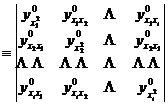
Calculate n determinants D 1 , D 2 ,..., D n sequentially for n variables . Then
( i ) A sufficient condition for the stable point x 0 to be a minimum point is that all determinants are positive, i.e.
D i >0 , i =1,2,![]()
( ii ) A sufficient condition for the stable point x 0 to be a maximum point is that all determinants with even numbers are positive, and all determinants with odd numbers are negative, that is
D i <0 , i =1,3,![]()
D i >0 , i =2,4,![]()
If neither of the above two conditions are satisfied, then the stable point may not be an extreme point . If all D i are zero, then higher order partial derivatives must be considered .
3 . Constraints are conditional extrema of the equation
find function
y = f ( x ) , x = ( x 1 , x 2 ) ![]()
at m ( m < n ) constraints
g k ( x )=0, k =1,2, ![]()
the extreme value below .
[ Direct substitution method ] Solve the m variables from the m equations of the constraints , represent them with the remaining n - m variables, and then directly substitute them into the function, so that it becomes a function that finds n - m variables The unconstrained extreme value problem of . This method is feasible if m variables can be solved from the constraint equations .
[ Lagrange Multiplier Method ] Introducing Modified Coefficients
F = y +![]()
where λ k is an undetermined constant . Taking F as an unconstrained function of n + m variables x 1 , x n and λ 1 , λ 2 , and finding the first-order partial derivatives of these variables to obtain the stable point of the equation :![]()
![]()
![]() , i =1, , n
, i =1, , n ![]()
g k = 0, k =1,2,![]()
Example 1 to find a function
y =![]()
under constraints
2 x 1 +3 x 2 =6
the extreme value below .
solution due to
y =![]()
and g = 2 x 1 +3 x 2 - 6=0
It can be seen that the modified function is
F = ( )+ λ ( 2 x 1 +3 x 2 - 6)![]()
solve system of equations
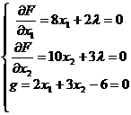
get λ = , x 1 = , x 2 = ![]()
![]()
![]()
So the stable point of the function F is
x 1 =, x 2 =![]()
![]()
Since D 1 == 8 > 0 ![]()
D 2 = =80>0![]()
This is a minimum point, and the minimum value of the function y is .![]()
[Penalty function method] Introduce a correction function when searching for a minimum point
F = y + (1)![]()
In the formula, P k is an arbitrarily large positive integer, which is called a penalty function . In this way, the problem can be transformed into an unconditional extreme value problem of a new function F , which can be minimized by increasing the value of P k . It can also be introduced as follows new function of the form![]()
F = y +![]()
where P k is an arbitrarily large positive integer .
When searching for the maximum point, take a negative sign before the penalty function, that is, introduce a new function
F = y −![]()
or F = y − ![]()
Example 2 Solve Example 1 using the penalty function method .
The solution uses equation ( 1 ) to introduce the correction function
F = y + P ( g ) 2 =![]()
solve system of equations

get x 1 = x 2 , x 2 = ![]()

When P is large, x 2 tends to , and x 1 tends to , which is the stable point . Since![]()
![]()
D 1 = =8(1+ P )>0![]()
D 2 = =16(5+14 P )>0![]()
So the stable point is a minimum point, which is consistent with the result of Example 1 .
4 . Constraints are conditional extremes of inequalities
A more general extremum problem than previously considered is to find the function
y = f ( x ) , x = ( x 1 , x 2 ,…, x n )
under m constraints
g k ( x )![]() , k =1,2,…, m
, k =1,2,…, m
The extreme value problem under , where m need not be less than n .
[ Slack variable method ] A non-negative slack function S i is introduced for each constraint inequality , and it becomes the equation:
![]() = g i + S i =0
= g i + S i =0
Each relaxation function S i depends only on one relaxation variable x n + i , generally taking
S i =![]()
After the relaxation function is introduced, the problem is transformed into an extreme value problem whose constraints are equations, and the previous method can be applied .
Example 3 to find a function
y =![]()
under constraints
x 1![]()
the extreme value below .
The solution constraints can be written as
g 1 =1- x 1![]()
Using the relaxation function S 1 ( x 3 ), this inequality can be constrained to an equation
![]() = g 1 + S 1 = x 1 +
= g 1 + S 1 = x 1 + ![]() =0
=0![]()
Using the direct substitution method, x 1 can be eliminated in the function y to get
y = 4(1+ ) 2 +5![]()
![]()
This is an unconstrained problem .
The stable point is x 2 =0, x 3 =0, so x 1 =1. Since
D 1 = =10>0![]()
D 2 = = =160>0
![]()
So the stable point is the minimum point of the modified and original function, and its minimum value is 4.
[ Lagrange Multiplier Method ] After introducing the relaxation function , the constraint inequalities are transformed into equations
![]() = g k + S k ( x n + k )=0, k =1, , m
= g k + S k ( x n + k )=0, k =1, , m ![]()
As in the case of equality constraints, introduce a new objective function
F = y +![]()
This is an unconstrained problem with n + 2 m variables . The stable point can be obtained by solving the following system of equations
![]() =0 , j =1, ,( n + m )
=0 , j =1, ,( n + m ) ![]()
![]() =0, k =1, , m
=0, k =1, , m ![]()
In the methods for finding the extremum and conditional extremum of the multivariate function described above, when finding the stable point, it all boils down to finding the real function equation system.
f I ( x 1 ,, x n )=0, i =1,, n![]()
![]()
A set of real roots of . Sometimes the real roots of the above equations are not easy to obtain, and approximate roots are required . For the approximate calculation method of real roots, please refer to Chapter 3, §4.
11. Application of Differentiation ( II ) - Character and Drawing of Curves
1. The properties of the curve and its conditions


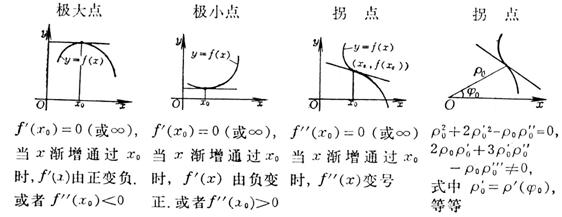
2. Singularity
Let P 0 ( x 0 , y 0 ) be the curve
F ( x , y )=0
a point on , assuming that the function F ( x , y ) has continuous partial derivatives at point P 0 and satisfies the condition
![]() ( x 0 , y 0 ) =0, ( x 0 , y 0 )=0
( x 0 , y 0 ) =0, ( x 0 , y 0 )=0![]()
Then P 0 is said to be a singular point of the curve F ( x , y )=0 .
If the second order partial derivatives of the function F ( x , y ) at the point P 0 ( x 0 , y 0 ) are not all zero, then P 0 is called a double point of the curve . Let
a = , b = , c =![]()
![]()
![]()
Then according to the sign of the discriminant, the following types of singularities can be divided into the two points .![]()
|
name and graphics |
condition and nature |
Example |
||||
|
Node
|
( i ) < 0 ( ii ) The curve has two branches passing through the point P 0 and has different tangents |
double kink
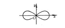
is based on the origin (0,0) as its node
|
||||
|
outlier
|
( i ) > 0 ( ii ) In a sufficiently small neighborhood of point P0 , there are no other points on the curve except point P0 . |
curve
The trajectory of is composed of the line x = 1 and the origin (0,0) , which is an isolated point of it |
|
|||
|
first point
name and graphics |
( i ) ( ii ) The curve consists of two branches with a common tangent at point P 0 , which are on the same side of their common normal and on opposite sides of the common tangent . condition and nature |
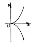
half cubic parabola
is the origin (0,0) as the first cusp Example |
|
|||
|
second cusp
|
( i ) ( ii ) The curve consists of two branches with a common tangent at point P 0 , which are on the same side of their common normal and on the same side of the common tangent . |
curve
There are two branches near the origin, namely
They have a common tangent at the origin. Since 0< x <1 , y always takes a positive value, so the two adjacent branches of the curve at the origin are on the same side of the common tangent and normal. |
|
|||
|
self cut point
|
( i ) ( ii ) The curve consists of two branches, which are tangent to each other at point P 0 |
curve
by two parabolas
composition, they are tangent to each other at the origin |
|
|||
If the curve consists of the parametric equation
x = x ( t ), y = y ( t )
|
Figure 5.9 |
It means that when =0 , =0 , the point ( x ( t 0 ), y ( t 0 )) determined by the parameter t 0 is the singularity of the curve .![]()
![]()
In particular, the curve is determined by the polar coordinate equation
![]()
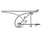
It means that when = =0 , the point ( , ) is the singularity of the curve . For example, when the hyperbolic spiral is ∞, =0 , so the pole is the singularity . When the polar angle increases to infinity, the point on the curve Infinitely approaches the pole, but cannot reach it (Fig. 5.9 ), so this singularity is also called asymptotic .![]()
![]()
![]()
![]()
![]()
![]()
![]()
![]()
3. Asymptote
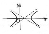
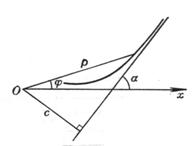
Condition and Asymptote Equation of Curve Existing Asymptote
|
Curve equation |
condition |
asymptote equation |
|
F ( x , y )=0 |
Denote the sum of terms of the highest degree of F ( x , y ) , and solve the equation = 0 , we get x =
Substitute y = kx + b into F ( x , y ) and expand by the power of x : F ( x , kx + b )= Solve Simultaneous Equations
Get k , b , which are the slope and vertical intercept of the asymptote |
x = a y = b y=kx + b |
|
y = f ( x ) |
|
y = kx + b x=a y=b |
|
|
|
y = kx + b x=a y=b |
|
|
|
|
4. Drawing
make a function
y =
f ( x )
The steps of the graph are roughly as follows:
(1) Determine the change interval of the independent variable x , and discuss some basic properties of the function, such as parity , symmetry and periodicity;
(2) Determine the intersection of the curve and the coordinate axis;
(3) Determine the vertex of the curve (maximum point , minimum point);
(4) Determine the convex part, concave part and inflection point of the curve;
(5) Determine the asymptote of the curve;
(6) Draw the dots for drawing .
Of course, specific issues need to be analyzed in detail, and the above points are not necessarily discussed .
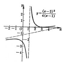
example curve
y =![]()
(1) x can vary over the interval ( -∞ , ∞ ) , is asymmetric, and has no parity and periodicity .
(2) Let x = 0, get y = ; let y = 0, get x = 3 ; That is, the curve and the coordinate axis intersect at the point (0, ), (3, 0) ( Figure 5.10).![]()
![]()
(3) Find the first-order and second-order derivatives , , and get the vertex (3,0) ( minimum point ) and![]()
![]()
( - 1 , - 2) ( maximum point ).
(4) The second derivative is positive when x > 1 and negative when x < 1. Therefore , the curve is concave in the interval (1, ∞ ) , and the curve is convex in the interval (- ∞ , 1) . Since the sign changes only when x = 1 , and this value of x corresponds to an asymptote parallel to the y -axis, there is no inflection point . ![]()
(5) When x = 1 , y becomes infinite, so this curve has an asymptote x = 1.
Find the asymptotes that are not parallel to the y -axis .
|
Figure 5.10 |
k =![]()
b =![]()
![]()
so y = ![]()
is an asymptote that is not parallel to the y -axis .
Draw a curve from these properties (Figure 5.10 ) .

