§ 4    Tensor Algorithms

 

1. The concept of tensor

 

    [ General definition of tensor ]   If a quantity has n ^N components, and the coordinate transformation of each component in the n -dimensional space R ⁿ

    ( i = 1 , ··· , n )

Below, it changes according to the following rules:

where is a function of x ⁱ , if yes , the quantity ( there are n ^N components in total ) is called the l -order contravariant ( or anti-variation ) m -order covariant N (= l + m ) -order mixed tensor ( or It is called a mixed tensor of type ( l + m ) .

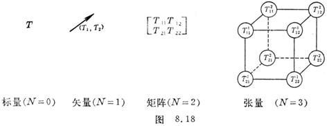
    The concept of tensors is a generalization of the concepts of vectors and matrices, scalars are zero-order tensors, vectors are first-order tensors, matrices ( square matrices ) are second-order tensors, and third-order tensors ( for example ) are like "stereo matrices" ( Figure 8.18 right ). Higher-order tensors cannot be expressed graphically . The following is a schematic diagram of tensors when n = 2 :

    [ Tensor example ]

    1 Multiplyable tensor Assuming that the two vectors a and b given by contravariant and covariant components are known, then the equation   

  All are second-order tensors, called multiplicative tensors .

    2   Kronecker notation The Kronecker notation is a second-order mixture tensor of first-order contravariant first-order covariance, since   

Available

    [ Second-order symmetric tensor and antisymmetric tensor ]   If the tensor satisfies the equation

are called the second-order symmetric covariant tensor, the second-order symmetric contravariant tensor, and the second-order symmetric mixture tensor, respectively . If the tensor satisfies the equation

are called second-order antisymmetric covariance tensors, second-order antisymmetric contravariant tensors, and second-order antisymmetric mixture tensors, respectively .

    The symmetric properties of contravariant ( covariant ) indices of tensors are invariant under coordinate transformations .

In three-dimensional space, a second-order antisymmetric tensor is equivalent to a vector .

 

2. Tensor Algebra

 

    [ Permutation of indicators ]   Permutation of indicators is the simplest operation of tensor algebra, and a new tensor can be made by using it . For example, through permutation of indicators, a new tensor can be obtained from a tensor , and its matrix is ​​the transformation of the matrix of the tensor. set matrix .

    [ Addition ( subtraction ) method ]   The corresponding components of several tensors of the same type are added ( or subtracted ) to obtain a new component of the same type of tensor. This operation is called tensor addition ( or subtraction ).

    Any second-order tensor can be decomposed into a symmetric tensor and an antisymmetric tensor . For example

    [ Multiplication of tensors ] Multiply   the components of two tensors according to various possible situations, and you will get the components of a new tensor . The order of contravariance and covariance of this tensor is equal to the original two tensors respectively. Sum of the order of contravariance and covariance of a quantity . This operation is called multiplication of tensors . For example       

This is a mixed tensor of order l + k contravariant m + h covariant of order l + m + k + h .

    Note that the order of tensor multiplication is not commutative .

    [ Contraction of tensors ]   For a given mixture tensor, add up a contravariant index and a covariant index equal to it, and get a lower order ( contravariance and covariance are one lower order each) ) , this operation is called contraction of tensors . For example

is a mixture tensor of order l - 1 contravariant and m - 1 covariant .

    [ Indicator rise and fall ]   In applications, the multiplication and contraction of second-order contravariant tensors are often used to "raise" the covariant index of tensors, and the multiplication and contraction of second-order covariant tensors are used to "lower" The contravariant index of the tensor . This operation is called the lifting and lowering of the index . For example, T _ijk can be raised and lowered by a ^ij and a _ij :

    [ quotient law of tensors ]   Let each sum be a function of a set of x ⁱ sums , if for any contravariant vector sum and any index j _k , let

and

If it becomes a tensor, it must be a tensor . This law of discriminating tensors is called the quotient law of tensors .

    For example , with a function of , and 

but

which is

holds for all , so the expression in the parentheses above equals zero, and is therefore a tensor .

    Substituting any covariant vector for the contravariant vector yields similar results .

    [ Tensor density ]   The quantity that changes according to the following rules

It is called tensor density, where it is a constant, which is called the weight of tensor density . A tensor is a tensor density with a weight of zero . According to the order of the tensor, scalar density and vector density can also be defined .

The sum of two tensor densities with the same number of indicators and the same weights is a tensor density of the same type . When two tensors are multiplied, the weights are added .

 

3. Tensor Analysis

 

    The above tensors all assume that their components are functions of a point M ( x ⁱ ) in the space R ⁿ :

When the point M ( x ⁱ ) changes in a certain area D in the space R ⁿ , it is called a tensor field in the area D. Various operations of the tensor algebra established above can be applied to the tensor Come on the field .

    There is also an invariant operation for tensor fields - absolute differentiation ( also known as covariant differentiation ) , which is what tensor analysis is about .

    The ordinary derivative of a scalar field is the component of a covariant vector field ( gradient field ) . However, in general, the ordinary derivative of a tensor field does not constitute a new tensor field .

    [ Affine contact space ]   If for each coordinate system ( x ⁱ ) in the space R ⁿ , a set of ( n ³ ) numbers are given at a known point M , and the coordinates are transformed

, they change according to the following rules

                       (1)

Then it is said that a contact object ( or contact coefficient ) is given at the point M , and the partial derivative takes the value at the point M.

    Suppose a contact object field is given in space R ⁿ

And these functions are continuously differentiable, then R ⁿ is called an affine connection space, denoted as L ⁿ . Generally speaking,

    [ torsion tensor ] The transformation law   in equation (1) includes two terms: the first term does not depend on the old coordinate system ; the second term depends on , and has the exact same form as the transformation law of the tensor . A term is symmetric to the two subscripts , it is generally not equal to zero, so it is not a tensor . But

constitute a tensor, called the torsion tensor of the affine connection space L n. If the torsion ^tensor is equal to zero, that is

Then the given space is said to be an affine connection space without torsion rate, denoted as .

    [ Absolute Differentiation and Parallel Movement of Vectors ] If   a contravariant vector is given in the space L ⁿ , under the coordinate transformation, there are

                               (2)

This constitutes the transformation law of the vector at point M. If we move from point M ( x ⁱ ) to point N ( x ⁱ + d x ⁱ ) , we have

where d a ⁱ represents the component of the change when the vector moves from M to N.

    Taking only one term in the above formula, we get

                             (3)

If the second partial derivative of the transformation is not equal to zero at M , then the amount of change in a vector is never a component of a vector .

    If R ⁿ is an affine connection space, it can be obtained from equations (1) , (2) and (3)

This indicates

is a contravariant infinitesimal vector . ^{Let Dai be the absolute differential of the vector at point M with respect to the displacement MN with component d x i} . If the object is contacted , the absolute differential ^agrees with the ordinary differential .

    If the vector is equal to zero, then

=0

It is said that the vector moves from point M to point N in parallel with respect to the connection . When the component a ⁱ remains unchanged (d a ⁱ = 0) , the vector moves from point M to point N in parallel , which is equivalent to the Euclidean space. Parallel movement .

    If given a curve C

x ⁱ = x ⁱ ( t )

and a contravariant vector , along this curve C can be made as the concomitant vector of

Call it the derivative along the curve C. If the derivative is zero, i.e.

                              (4)

Then the vector a ⁱ moves parallel to the curve C , the formula (4) has nothing to do with the choice of the coordinate system, that is to say, the parallel movement of the vector along the curve is unchanged under the coordinate transformation .

    Similarly, absolute differentiation and parallel movement of covariant vectors can be considered .

is the absolute differential of the covariant vector with respect to the displacement d x ⁱ . The condition for parallel movement is

Or the condition for parallel movement along the curve C is

    [ Covariant Derivative ]   From the definition formula of the absolute differential of contravariant vector and covariant vector, the quantity can be obtained

and

They are second-order tensors covariant with respect to the index k , called the covariant derivatives of the vector sums, denoted sum or sum , respectively .

    [ Absolute Differentiation and Parallel Shift of Tensor and Its Covariant Differential Method ]

    From the differential formula of the product and the definition of the tensor, the law of parallel movement of the tensor can be deduced .

    For example, the parallel movement law of a third-order tensor is

The parallel movement law of the fourth-order tensor is:

It can be seen that the number of items contained in the law of parallel movement of tensor is the same as the order of tensor . For the contravariant index of tensor , it is similar to the law of parallel movement of contravariant vector ; for the covariant index of tensor , similar to the law of parallel movement of covariant vectors .

is called the absolute differential of a tensor .

    [ Covariant derivatives of tensors and their algorithms ]

is called the covariant derivative of a tensor, which is a component of a fifth-order tensor .

    In the ordinary derivative, adding an item to each index of the differentiated tensor can form the covariant derivative of any tensor. For the contravariant index, the form of this term is

For the covariance indicator is

    The algorithm for covariant derivatives is as follows:

    1 The covariant derivative of the sum of several tensors of the same structure is equal to the sum of the covariant derivatives of each tensor, that is 

    2   Satisfy the differential law of the product, that is

    [ Self-parallel curve ] In the affine connection space, if   every vector tangent to a point M ₀ on the curve is tangent to the curve when moving in parallel along the curve, the curve is called a self-parallel curve .

    Let the equation of the curve be x ⁱ = x ⁱ ( t ), its tangent vector is , the condition of its parallel movement along the curve is

This is the differential equation of the connected self-parallel curve . Let

The above differential equation can be written as

The coefficients are obviously symmetric with respect to j and k , and constitute an affine connection . It is said to constitute a symmetric affine connection associated with , if it is also symmetric with respect to j and k , it is consistent with .